http://www.dip.ee.uct.ac.za/~nicolls/lectures/eee4001f/

http://ft-sipil.unila.ac.id/dbooks/The%20Scientist%20and%20Engineer's%20Guide%20to%20Digital%20Signal%20Process.pdf

http://s-mat-pcs.oulu.fi/~ssa/ESignals/em4_5-1.htm
http://dsp-book.narod.ru/HFTSP/8579ch15.pdf
http://www.katjaas.nl/hilbert/hilbert.html
http://www.mikrocontroller.net/attachment/33905/Audio_Hilbert_WAR19.pdf
http://w3.msi.vxu.se/exarb/mj_ex.pdf
http://en.wikipedia.org/wiki/Hilbert_transform
http://www.hitech.technion.ac.il/~feldman/hilbert2.html
http://dsp.stackexchange.com/questions/424/hilbert-transform-to-compute-signal-envelope

Hilbert transform

From Wikipedia, the free encyclopedia

In mathematics and in signal processing, the Hilbert transform is a linear operator which takes a function, u(t), and produces a function, H(u)(t), with the same domain. The Hilbert transform is named after David Hilbert, who first introduced the operator in order to solve a special case of the Riemann–Hilbert problem for holomorphic functions. It is a basic tool in Fourier analysis, and provides a concrete means for realizing the harmonic conjugate of a given function or Fourier series. Furthermore, inharmonic analysis, it is an example of a singular integral operator, and of a Fourier multiplier. The Hilbert transform is also important in the field of signal processing where it is used to derive the analytic representation of a signal u(t).

The Hilbert transform was originally defined for periodic functions, or equivalently for functions on thecircle, in which case it is given by convolution with the Hilbert kernel. More commonly, however, the Hilbert transform refers to a convolution with the Cauchy kernel, for functions defined on the real line R(the boundary of the upper half-plane). The Hilbert transform is closely related to the Paley–Wiener theorem, another result relating holomorphic functions in the upper half-plane and Fourier transforms of functions on the real line.

The Hilbert transform, in red, of a square wave, in blue

[edit]Introduction

The Hilbert transform of u can be thought of as the convolution of u(t) with the function h(t) = 1/(π t). Because h(t) is not integrable the integrals defining the convolution do not converge. Instead, the Hilbert transform is defined using the Cauchy principal value (denoted here by p.v.) Explicitly, the Hilbert transform of a function (or signal) u(t) is given by

$H(u)(t) = \text{p.v.} \int_{-\infty}^{\infty}u(\tau) h(t-\tau)\, d\tau =\frac{1}{\pi} \ \text{p.v.} \int_{-\infty}^{\infty} \frac{u(\tau)}{t-\tau}\, d\tau,$

provided this integral exists as a principal value. This is precisely the convolution of u with the tempered distribution p.v. 1/πt (due to Schwartz (1950); see Pandey (1996, Chapter 3)). Alternatively, by changing variables, the principal value integral can be written explicitly (Zygmund 1968, §XVI.1) as

$H(u)(t) = -\frac{1}{\pi}\lim_{\varepsilon\downarrow 0}\int_{\varepsilon}^\infty \frac{u(t+\tau)-u(t-\tau)}{\tau}\,d\tau.$

When the Hilbert transform is applied twice in succession to a function u, the result is negative u:

$H(H(u))(t) = -u(t),\,$

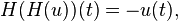
provided the integrals defining both iterations converge in a suitable sense. In particular, the inverse transform is −H. This fact can most easily be seen by considering the effect of the Hilbert transform on the Fourier transform of $u(t)$ (see Relationship with the Fourier transform, below).

For an analytic function in upper half-plane the Hilbert transform describes the relationship between the real part and the imaginary part of the boundary values. That is, if f(z) is analytic in the plane Im z > 0 andu(t) = Re f(t + 0·i ) then Im f(t + 0·i ) = H(u)(t) up to an additive constant, provided this Hilbert transform exists.

[edit]Notation

This section does not cite anyreferences or sources.(December 2011)

In signal processing the Hilbert transform of u(t) is commonly denoted by $\widehat u(t).\,$ However, in mathematics, this notation is already extensively used to denote the Fourier transform of u(t). Occasionally, the Hilbert transform may be denoted by $\tilde{u}(t)$ . Furthermore, many sources define the Hilbert transform as the negative of the one defined here.

[edit]History

The Hilbert transform arose in Hilbert's 1905 work on a problem posed by Riemann concerning analytic functions (Kress (1989); Bitsadze (2001)) which has come to be known as the Riemann–Hilbert problem. Hilbert's work was mainly concerned with the Hilbert transform for functions defined on the circle (Khvedelidze 2001; Hilbert 1953). Some of his earlier work related to the Discrete Hilbert Transform dates back to lectures he gave in Göttingen. The results were later published by Hermann Weyl in his dissertation (Hardy, Littlewood & Polya 1952, §9.1). Schur improved Hilbert's results about the discrete Hilbert transform and extended them to the integral case (Hardy, Littlewood & Polya 1952, §9.2). These results were restricted to the spaces L² and ℓ². In 1928, Marcel Riesz proved that the Hilbert transform can be defined for u in L^p(R) for 1 < p < ∞, that the Hilbert transform is a bounded operator on L^p(R) for the same range of p, and that similar results hold for the Hilbert transform on the circle as well as the discrete Hilbert transform (Riesz 1928). The Hilbert transform was a motivating example for Antoni Zygmund and Alberto Calderón during their study of singular integrals (Calderón & Zygmund 1952). Their investigations have played a fundamental role in modern harmonic analysis. Various generalizations of the Hilbert transform, such as the bilinear and trilinear Hilbert transforms are still active areas of research today.

[edit]Relationship with the Fourier transform

The Hilbert transform is a multiplier operator (Duoandikoetxea 2000, Chapter 3). The symbol of H is σ_H(ω) = −i sgn(ω) where sgn is the signum function. Therefore:

$\mathcal{F}(H(u))(\omega) = (-i\,\operatorname{sgn}(\omega))\cdot \mathcal{F}(u)(\omega)\,$

where $\mathcal{F}$ denotes the Fourier transform. Since sgn(x) = sgn(2πx), it follows that this result applies to the three common definitions of $\mathcal{F}.$

By Euler's formula,

$\sigma_H(\omega) \, \ =\ \begin{cases} \ \ i = e^{+i\pi/2}, & \mbox{for } \omega < 0\\ \ \ \ \ 0, & \mbox{for } \omega = 0\\ \ \ -i = e^{-i\pi/2}, & \mbox{for } \omega > 0. \end{cases}$

Therefore H(u)(t) has the effect of shifting the phase of the negative frequency components of u(t) by +90° (π/2 radians) and the phase of the positive frequency components by −90°. And i·H(u)(t) has the effect of restoring the positive frequency components while shifting the negative frequency ones an additional +90°, resulting in their negation.

When the Hilbert transform is applied twice, the phase of the negative and positive frequency components of u(t) are respectively shifted by +180° and −180°, which are equivalent amounts. The signal is negated, i.e., H(H(u)) = −u, because:

$\big(\sigma_H(\omega)\big)^2 = e^{\pm i\pi} = -1 \qquad \text{for } \omega\neq 0.$

[edit]Table of selected Hilbert transforms

Signal $u(t)\,$	Hilbert transform^{[fn 1]} $H(u)(t)\,$
$\sin(t)\,$ ^{[fn 2]}	$-\cos(t)\,$
$\cos(t)\,$ ^{[fn 2]}	$\sin(t)\,$
$\exp \left( i t \right)$	$- i \exp \left( i t \right)$
$\exp \left( -i t \right)$	$i \exp \left( -i t \right)$
$1 \over t^2 + 1$	$t \over t^2 + 1$
Sinc function $\sin(t) \over t$	$1- \cos(t)\over t$
Rectangular function 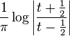$\sqcap(t)$	${1 \over \pi} \log \left \| {t+{1 \over 2} \over t-{1 \over 2}} \right \|$
Dirac delta function $\delta(t) \,$	${1 \over \pi t}$
Characteristic Function $\chi_{[a,b]}(t) \,$	$\frac{1}{\pi}\log \left \vert \frac{t-a}{t-b}\right \vert \,$

Notes

^ Some authors, e.g., Bracewell, use our −H as their definition of the forward transform. A consequence is that the right column of this table would be negated.
^ ^a ^b The Hilbert transform of the sin and cos functions can be defined in a distributional sense, if there is a concern that the integral defining them is otherwise conditionally convergent. In the periodic setting this result holds without any difficulty.

An extensive table of Hilbert transforms is available (King 2009). Note that the Hilbert transform of a constant is zero.

[edit]Domain of definition

It is by no means obvious that the Hilbert transform is well-defined at all, as the improper integral defining it must converge in a suitable sense. However, the Hilbert transform is well-defined for a broad class of functions, namely those in L^p(R) for 1<p<∞.

More precisely, if u is in L^p(R) for 1<p<∞, then the limit defining the improper integral

$H(u)(t) = -\frac{1}{\pi}\lim_{\epsilon\downarrow 0}\int_\epsilon^\infty \frac{u(t+\tau)-u(t-\tau)}{\tau}\,d\tau$

exists for almost every t. The limit function is also in L^p(R), and is in fact the limit in the mean of the improper integral as well. That is,

$-\frac{1}{\pi}\int_\epsilon^\infty \frac{u(t+\tau)-u(t-\tau)}{\tau}\,d\tau\to H(u)(t)$

as ε→0 in the L^p-norm, as well as pointwise almost everywhere, by the Titchmarsh theorem (Titchmarsh 1948, Chapter 5).

In the case p=1, the Hilbert transform still converges pointwise almost everywhere, but may fail to be itself integrable even locally (Titchmarsh 1948, §5.14). In particular, convergence in the mean does not in general happen in this case. The Hilbert transform of an L¹ function does converge, however, in L¹-weak, and the Hilbert transform is a bounded operator from L¹ to L^1,w (Stein & Weiss 1971, Lemma V.2.8). (In particular, since the Hilbert transform is also a multiplier operator on L², Marcinkiewicz interpolation and a duality argument furnishes an alternative proof that H is bounded on L^p.)

MY WORLD

Wednesday, November 14, 2012