http://www.youtube.com/watch?v=Bf66VrekSKc
Monday, May 28, 2012
Create a Bootable Linux Flash Drive form iso file
Create a Bootable Linux Flash Drive in
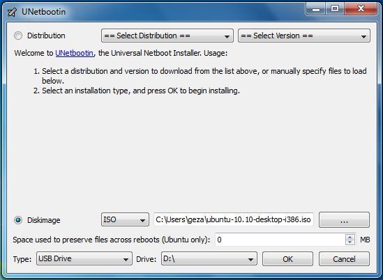
Just download and run the program, then choose a Linux distribution (i.e. a version of Linux) or, if you already have one, an ISO file. I think most people will opt for the former, at which point UNetbootin downloads Linux for you, then copies it to your flash drive (and makes the drive bootable).
(If you're new to Linux, I recommend choosing Ubuntu--though readers may have other ideas as to which distribution is the most user-friendly.)
Reboot with your drive still inserted and presto: Linux should load. (You may need to monkey with your BIOS or boot settings so that the flash drive is at the top of the order.)
Keep in mind that this won't overwrite anything on your hard drive; the OS runs exclusively from the flash drive. When you're done, you can just shut down, remove the drive, then boot back into Windows normally.
But I recommend familiarizing yourself with that Linux environment, just so you're prepared if and when you need to use it for rescue purposes. Plus, it's kind of fun!
_________________________________________________________________________________
Burn ISO Image to USB Flash Pen Drive (Kon-Boot to USB)
http://www.raymond.cc/blog/burn-iso-image-to-usb-flash-pen-drive-kon-boot-to-usb/
When I discovered Kon-Boot and posted it in this blog, I got many request in forum on how to put Kon-Boot ISO image file to USB. I seldom boot a computer using USB because only modern computers is able to support that and a lot of my client’s computer are still old enough to only support booting from CD. Booting up a computer with USB is very convenient because USB is small, cheap and convenient. Imagine carrying a small pendrive with Kon-Boot and you can virtually login to any password protected Windows or Linux computer…
Many of you tried to extract the Kon-Boot ISO image file but ended up seeing that it’s blank. The image file is NOT blank and even the coder of Kon-Boot mentions that. It’s just that you can’t see it in Windows. For those that are having trouble in putting Kon-Boot ISO to USB, I will show you how easy it is to do that. Remember, computers are made easy in Raymond.CC ;)
There are 2 types of Kon-Boot images. The floppy image and CD ISO. You can use UNetbootin, a tool that allows you to create bootable Live USB drives for a variety of Linux distributions from Windows or Linux, without requiring you to burn a CD. The trick here is to use the floppy image instead of the CD ISO. If you don’t get what am I saying, just follow the few simple step-by-step on how to burn Kon-Boot ISO to USB.
1. Download latest version of UNetbootin and install.
2. Download Kon-Boot floppy image and extract the zip file to get FD0-konboot-v1.1-2in1.img file.
3. Plug in your USB flash drive.
4. Run UNetbootin, select Diskimage, click the drop down menu to select Floppy and browse for the FD0-konboot-v1.1-2in1.img file.

5. Make sure USB Drive is selected for Type and the drive letter is the USB flash drive that you want to install Kon-Boot. Click OK. It should take a few seconds to finish installing Kon-Boot floppy image into your USB.
6. You can click the Reboot Now button and boot up your computer with USB. You may have to set your BIOS to do that. On newer computers, there should be a hotkey to show the Boot Menu. My MSI motherboard hotkey is F8.
7. If you get it right, you should see a UNetbootin screen with 10 seconds countdown to select Default from the list. You can either hit enter to immediately boot Kon-Boot or just wait until 10 seconds for UNetbootin to automatically boot the default profile for you.

8. When you see the Krypto Logic screen, hit a key to continue. Just wait for Windows or Linux to boot normally. Now you can login to any user account without entering a password!
I have no idea why UNetbootin doesn’t work with Kon-Boot CD ISO image file, maybe it is not compatible. However, you can see that UNetbootin supports a pretty good amount of linux distros and possibly other ISO that is not in the list. Well at least we got Kon-Boot into USB thanks to the floppy image file.
Setting up http-proxy in ubuntu and fedora
In fedora ,centos,fuduntu
http://www.centos.org/docs/5/html/yum/sn-yum-proxy-server.html
10. Using yum with a Proxy Server
By default, yum accesses network repositories
with HTTP. All yum HTTP operations use
HTTP/1.1, and are compatible with web proxy servers that support
this standard. You may also access FTP repositories, and configure
yum to use an FTP proxy server. The
squid package provides a proxy service for
both HTTP/1.1 and FTP connections.
![[Tip]](http://www.centos.org/HEADER.images/tip.png) | Modifying yum for Network Compatibility |
|---|---|
Refer to the man page for
yum.conf for information on HTTP settings
that may be modified for compatibility with nonstandard web
proxy servers. Alternatively, configure yum
to use an FTP proxy server, and access repositories that support
FTP. The Fedora repositories support both HTTP and FTP.
|
To enable all
The settings below enable
yum operations to use a proxy
server, specify the proxy server details in
/etc/yum.conf. The proxy
setting must specify the proxy server as a complete URL,
including the TCP port number. If your proxy server requires a
username and password, specify these by adding
proxy_username and
proxy_password settings.
The settings below enable
yum to use the
proxy server
mycache.mydomain.com,
connecting to port 3128, with the username
yum-user and the
password qwerty.
# The proxy server - proxy server:port number
proxy=http://mycache.mydomain.com:3128
# The account details for yum connections
proxy_username=yum-user
proxy_password=qwerty
Example 3. Configuration File Settings for Using A Proxy Server
10.2. Configuring Proxy Server Access for a Single User
bash shell, the profile is the file
~/.bash_profile. The settings below enable
yum to use the proxy server
mycache.mydomain.com,
connecting to port 3128.
# The Web proxy server used by this account
http_proxy="http://mycache.mydomain.com:3128"
export http_proxy
Example 4. Profile Settings for Using a Proxy Server
yum-user and the
password qwerty, add these settings:
# The Web proxy server, with the username and password for this account
http_proxy="http://yum-user:qwerty@mycache.mydomain.com:3128"
export http_proxy
Example 5. Profile Settings for a Secured Proxy Server
______________________________________________________________________
In case of UBUNTU
https://help.ubuntu.com/community/AptGet/Howto
Setting up apt-get to use a http-proxy
These are three methods of using apt-get with a http-proxy.
Temporary proxy session
This is a
temporary method that you can manually use each time you want to use
apt-get through a http-proxy. This method is useful if you only want to
temporarily use a http-proxy.
Enter this line in the terminal prior to using apt-get (substitute your details for yourproxyaddress and proxyport).
export http_proxy=http://yourproxyaddress:proxyport
If
you normally use sudo to run apt-get you will need to login as root
first for this to work unless you also add some explicit environment
settings to /etc/sudoers, e.g.
Defaults env_keep = "http_proxy https_proxy ftp_proxy"
APT configuration file method
This method uses the apt.conf file which is found in your /etc/apt/ directory. This method is useful if you only want apt-get (and not other applications) to use a http-proxy permanently.
 On some installations there will be no apt-conf file set up. This
procedure will either edit an existing apt-conf file or create a new
apt-conf file.
On some installations there will be no apt-conf file set up. This
procedure will either edit an existing apt-conf file or create a new
apt-conf file. |
gksudo gedit /etc/apt/apt.conf
Add this line to your /etc/apt/apt.conf file (substitute your details for yourproxyaddress and proxyport).
Acquire::http::Proxy "http://yourproxyaddress:proxyport";
Save the apt.conf file.
BASH rc method
This method
adds a two lines to your .bashrc file in your $HOME directory. This
method is useful if you would like apt-get and other applications for
instance wget, to use a http-proxy.
gedit ~/.bashrc
Add these lines to the bottom of your ~/.bashrc file (substitute your details for yourproxyaddress and proxyport)
http_proxy=http://yourproxyaddress:proxyport
export http_proxy
Save the file. Close your terminal window and then open another terminal window or source the ~/.bashrc file:
source ~/.bashrc
Test
your proxy with sudo apt-get update and whatever networking tool you
desire. You can use firestarter or conky to see active connections.
If you make a mistake and go back to edit the file again, you can close the terminal and reopen it or you can source ~/.bashrc as shown above.
source ~/.bashrc
How to login a proxy user
If you need
to login to the Proxy server this can be achieved in most cases by
using the following layout in specifying the proxy address in
http-proxy. (substitute your details for username, password, yourproxyaddress and proxyport)
http_proxy=http://username:password@yourproxyaddress:proxyport
ref
http://www.ubuntugeek.com/how-to-configure-ubuntu-desktop-to-use-your-proxy-server.html
http://support.citrix.com/article/CTX132001
Saturday, May 26, 2012
video filter and processing
http://en.wikipedia.org/wiki/Filter_%28video%29
A video filter is a software component that is used to decode audio and video.[1] Multiple filters can be used in a filter chain, in which each filter receives input from its previous-in-line filter upstream[disambiguation needed ], processes the input and outputs the processed video to its next-in-line filter downstream[disambiguation needed ]. Such a configuration can be visualized in a filter graph.
With regards to video encoding three categories of filters can be distinguished:
The following figures are from A.M. Tekalp, "Digital video processing", Prentice Hall PTR, 1995, NTSC.
The video scanning formats supported by the ATSC Digital Television Standard are shown in the following table.
book
http://eeweb.poly.edu/~yao/videobook/
Introduction
The purpose of this lab is to acquaint you with the TI Image Developers Kit (IDK). The IDK contains a floating point C6711 DSP, and other hardware that enables real time video/image processing. In addition to the IDK, the video processing lab bench is equipped with an NTSC camera and a standard color computer monitor.
You will complete an introductory exercise to gain familiarity with the IDK programming environment. In the exercise, you will modify a C skeleton to horizontally flip and invert video input (black and white) from the camera. The output of your video processing algorithm will appear in the top right quadrant of the monitor.
In addition, you will analyze existing C code that implements filtering and edge detection algorithms to gain insight into IDK programming methods. The output of these "canned" algorithms, along with the unprocessed input, appears in the other quadrants of the monitor.
Finally, you will create an auto contrast function. And will also work with a color video feed and create a basic user interface, which uses the input to control some aspect of the display.
An additional goal of this lab is to give you the opportunity to discover tools for developing an original project using the IDK.
Important Documentation
The following documentation will certainly prove useful:
The IDK
User's Guide. Section 2 is the most important. The IDK
Video Device Drivers User's Guide. The sections on timing are not too important, but pay attention to the Display and Capture systems and have a good idea of how they work. The IDK
Programmer's Guide. Sections 2 and 5 are the ones needed. Section 2 is very, very important in Project Lab 2. It is also useful in understanding “streams” in project lab 1.
Note: Other manuals may be found on TI's website by searching for
TMS320C6000 IDK
Video Processing - The Basics
The camera on the video processing lab bench generates a video signal in NTSC format. NTSC is a standard for transmitting and displaying video that is used in television. The signal from the camera is connected to the "composite input" on the IDK board (the yellow plug). This is illustrated in Figure 2-1 on page 2-3 of the IDK User's Guide. Notice that the IDK board is actually two boards stacked on top of each other. The bottom board contains the C6711 DSP, where your image processing algorithms will run. The daughterboard is on top, it contains the hardware for interfacing with the camera input and monitor output. For future video processing projects, you may connect a video input other than the camera, such as the output from a DVD player. The output signal from the IDK is in RGB format, so that it may be displayed on a computer monitor.
At this point, a description of the essential terminology of the IDK environment is in order. The video input is first decoded and then sent to the FPGA, which resides on the daughterboard. The FPGA is responsible for video capture and for the filling of the input frame buffer (whose contents we will read). For a detailed description of the FPGA and its functionality, we advise you to read Chapter 2 of the IDK User's Guide.
The Chip Support Library (CSL) is an abstraction layer that allows the IDK daughterboard to be used with the entire family of TI C6000 DSPs (not just the C6711 that we're using); it takes care of what is different from chip to chip.
The Image Data Manager (IDM) is a set of routines responsible for moving data between on-chip internal memory, and external memory on the board, during processing. The IDM helps the programmer by taking care of the pointer updates and buffer management involved in transferring data. Your DSP algorithms will read and write to internal memory, and the IDM will transfer this data to and from external memory. Examples of external memory include temporary "scratch pad" buffers, the input buffer containing data from the camera, and the output buffer with data destined for the RGB output.
The two different memory units exist to provide rapid access to a larger memory capacity. The external memory is very large in size – around 16 MB, but is slow to access. But the internal is only about 25 KB or so and offers very fast access times. Thus we often store large pieces of data, such as the entire input frame, in the external memory. We then bring it in to internal memory, one small portion at a time, as needed. A portion could be a line or part of a line of the frame. We then process the data in internal memory and then repeat in reverse, by outputting the results line by line (or part of) to external memory. This is full explained in Project Lab 2, and this manipulation of memory is important in designing efficient systems.
The TI C6711 DSP uses a different instruction set than the 5400 DSP's you are familiar with in lab. The IDK environment was designed with high level programming in mind, so that programmers would be isolated from the intricacies of assembly programming. Therefore, we strongly suggest that you do all your programming in C. Programs on the IDK typically consist of a main program that calls an image processing routine.
The main program serves to setup the memory spaces needed and store the pointers to these in objects for easy access. It also sets up the input and output channels and the hardware modes (color/grayscale ...). In short it prepares the system for our image processing algorithm.
The image processing routine may make several calls to specialized functions. These specialized functions consist of an outer wrapper and an inner component. The wrapper oversees the processing of the entire image, while the component function works on parts of an image at a time. And the IDM moves data back and forth between internal and external memory.
As it brings in one line in from external memory, the component function performs the processing on this one line. Results are sent back to the wrapper. And finally the wrapper contains the IDM instructions to pass the output to external memory or wherever else it may be needed.
Please note that this is a good methodology used in programming for the IDK. However it is very flexible too, the "wrapper" and "component functions" are C functions and return values, take in parameters and so on too. And it is possible to extract/output multiple lines or block etc. as later shown.
In this lab, you will modify a component to implement the flipping and inverting algorithm. And you will perform some simple auto-contrasting as well as work with color.
In addition, the version of Code Composer that the IDK uses is different from the one you have used previously. The IDK uses Code Composer Studio v2.1. It is similar to the other version, but the process of loading code is slightly different.
Code DescriptionOverview and I/O
The next few sections describe the code used. First please copy the files needed by following the instructions in the "Part 1" section of this document. This will help you easily follow the next few parts.
The program flow for image processing applications may be a bit different from your previous experiences in C programming. In most C programs, the main function is where program execution starts and ends. In this real-time application, the main function serves only to setup initializations for the cache, the CSL, and the DMA (memory access) channel. When it exits, the main task, tskMainFunc(), will execute automatically, starting the DSP/BIOS. It will loop continuously calling functions to operate on new frames and this is where our image processing application begins.
The tskMainFunc(), in main.c, opens the handles to the board for image capture (VCAP_open()) and to the display (VCAP_open()) and calls the grayscale function. Here, several data structures are instantiated that are defined in the file img_proc.h. The IMAGE structures will point to the data that is captured by the FPGA and the data that will be output to the display. The SCRATCH_PAD structure points to our internal and external memory buffers used for temporary storage during processing. LPF_PARAMS is used to store filter coefficients for the low pass filter.
The call to img_proc() takes us to the file img_proc.c. First, several variables are declared and defined. The variable quadrant will denote on which quadrant of the screen we currently want output; out_ptr will point to the current output spot in the output image; and pitch refers to the byte offset (distance) between two lines. This function is the high level control for our image-processing algorithm. See algorithm flow.
Figure 1: Algorithm FlowFigure 1 (video1.jpg)
The first function called is the pre_scale_image function in the file pre_scale_image.c. The purpose of this function is to take the 640x480 image and scale it down to a quarter of its size by first downsampling the input rows by two and then averaging every two pixels horizontally. The internal and external memory spaces, pointers to which are in the scratch pad, are used for this task. The vertical downsampling occurs when every other line is read into the internal memory from the input image. Within internal memory, we will operate on two lines of data (640 columns/line) at a time, averaging every two pixels (horizontal neighbors) and producing two lines of output (320 columns/line) that are stored in the external memory.
To accomplish this, we will need to take advantage of the IDM by initializing the input and output streams. At the start of the function, two instantiations of a new structure dstr_t are declared. You can view the structure contents of dstr_t on p. 2-11 of the IDK Programmer's Guide. These structures are stream "objects". They give us access to the data when using the dstr_open() command. In this case dstr_i is an input stream as specified in the really long command dstr_open(). Thus after opening this stream we can use the get_data command to get data one line at a time. Streams and memory usage are described in greater detail in the second project lab. This data flow for the pre-scale is shown in data flow.
Figure 2: Data flow of input and output streams.Figure 2 (video2.jpg)
To give you a better understanding of how these streams are created, let's analyze the parameters passed in the first call to dstr_open() which opens an input stream.
External address: in_image->data
This is a pointer to the place in external memory serving as the source of our input data (it's the source because the last function parameter is set to DSTR_INPUT). We're going to bring in data from external to internal memory so that we can work on it. This external data represents a frame of camera input. It was captured in the main function using the VCAP_getframe() command.
External size: (rows + num_lines) * cols = (240 + 2) * 640
This is the total size of the input data which we will bring in. We will only be taking two lines at a time from in_image->data, so only 240 rows. The "plus 2" represents two extra rows of input data which represent a buffer of two lines - used when filtering, which is explained later.
Internal address: int_mem
This is a pointer to an 8x640 array, pointed to by scratchpad->int_data. This is where we will be putting the data on each call to dstr_get(). We only need part of it, as seen in the next parameter, as space to bring in data.
Internal size: 2 * num_lines * cols = 2 * 2 * 640
The size of space available for data to be input into int_mem from in_image->data. We pull in two lines of the input frame so it num_lines * cols. We have the multiply by 2 as we are using double buffering for bringing in the data. We need double the space in internal memory than the minimum needed, the reason is fully explained in IDK Programmer's Guide.
Number of bytes/line: cols = 640, Number of lines: num_lines = 2
Each time dstr_get_2D() is called, it will return a pointer to 2 new lines of data, 640 bytes in length. We use the function dstr_get_2D(), since we are pulling in two lines of data. If instead we were only bringing in one line, we would use dstr_get() statements.
External memory increment/line: stride*cols = 1*640
The IDM increments the pointer to the external memory by this amount after each dstr_get() call.
Window size: 1 for double buffered single line of data
(Look at the three documentation pdfs for a full explanation of double buffering)
The need for the window size is not really apparent here.
It will become apparent when we do the 3x3 block convolution. Then, the window size will be set to 3 (indicating three lines of buffered data). This tells the IDM to send a pointer to extract 3 lines of data when dstr_get() is called, but only increment the stream's internal pointer by 1 (instead of 3) the next time dstr_get() is called. Thus you will get overlapping sets of 3 lines on each dstr_get() call. This is not a useful parameter when setting up an output stream.
Direction of input: DSTR_INPUT
Sets the direction of data flow. If it had been set to DSTR_OUTPUT (as done in the next call to dstr_open()), we would be setting the data to flow from the Internal Address to the External Address.
We then setup our output stream to write data to a location in external memory which we had previously created.
Once our data streams are setup, we can begin processing by first extracting a portion of input data using dstr_get_2D(). This command pulls the data in and we setup a pointer (in_data) to point to this internal memory spot. We also get a pointer to a space where we can write the output data (out_data) when using dstr_put(). Then we call the component function pre_scale() (in pre_scale.c) to operate on the input data and write to the output data space, using these pointers.
The prescaling function will perform the horizontal scaling by averaging every two pixels. This algorithm operates on four pixels at a time. The entire function is iterated within pre_scale_image() 240 times, which results in 240 * 2 rows of data being processed – but only half of that is output.
Upon returning to the wrapper function, pre_scale_image, a new line is extracted; the pointers are updated to show the location of the new lines and the output we had placed in internal memory is then transferred out. This actually happens in the dstr_put() function – thus is serves a dual purpose; to give us a pointer to internal memory which we can write to, and the transferring of its contents to external memory.
Before pre_scale_image() exits, the data streams are closed, and one line is added to the top and bottom of the image to provide context necessary for the next processing steps (The extra two lines - remember?). Also note, it is VERY important to close streams after they have been used.
If not done, unusual things such as random crashing and so may occur which are very hard to track down.
Now that the input image has been scaled to a quarter of its initial size, we will proceed with the four image processing algorithms. In img_proc.c, the set_ptr() function is called to set the variable out_ptr to point to the correct quadrant on the 640x480 output image. Then copy_image(), copy_image.c, is called, performing a direct copy of the scaled input image into the lower right quadrant of the output.
Next we will set the out_ptr to point to the upper right quadrant of the output image and call conv3x3_image() in conv3x3_image.c. As with pre_scale_image(), the _image indicates this is only the wrapper function for the ImageLIB (library functions) component, conv3x3(). As before, we must setup our input and output streams. This time, however, data will be read from the external memory (where we have the pre-scaled image) and into internal memory for processing, and then be written to the output image. Iterating over each row, we compute one line of data by calling the component function conv3x3() in conv3x3.c.
In conv3x3(), you will see that we perform a 3x3 block convolution, computing one line of data with the low pass filter mask. Note here that the variables IN1[i], IN2[i], and IN3[i] all grab only one pixel at a time. This is in contrast to the operation of pre_scale() where the variable in_ptr[i] grabbed 4 pixels at a time. This is because in_ptr was of type unsigned int, which implies that it points to four bytes (the size of an unsigned int is 4 bytes) of data at a time. IN1, IN2, and IN3 are all of type unsigned char, which implies they point to a single byte of data. In block convolution, we are computing the value of one pixel by placing weights on a 3x3 block of pixels in the input image and computing the sum. What happens when we are trying to compute the rightmost pixel in a row? The computation is now bogus. That is why the wrapper function copies the last good column of data into the two rightmost columns. You should also note that the component function ensures output pixels will lie between 0 and 255. For the same reason we provided the two extra "copied" lines when performing the prescale.
Back in img_proc.c, we can begin the edge detection algorithm, sobel_image(), for the lower left quadrant of the output image. This wrapper function, located in sobel_image.c, performs edge detection by utilizing the assembly written component function sobel() in sobel.asm. The wrapper function is very similar to the others you have seen and should be straightforward to understand. Understanding the assembly file is considerably more difficult since you are not familiar with the assembly language for the c6711 DSP. As you'll see in the assembly file, the comments are very helpful since an "equivalent" C program is given there.
The Sobel algorithm convolves two masks with a 3x3 block of data and sums the results to produce a single pixel of output. One mask has a preference for vertical edges while the other mask for horizontal ones. This algorithm approximates a 3x3 nonlinear edge enhancement operator. The brightest edges in the result represent a rapid transition (well-defined features), and darker edges represent smoother transitions (blurred or blended features).
Part One
This section provides a hands-on introduction to the IDK environment that will prepare you for the lab exercise. First, connect the power supply to the IDK module. Two green lights on the IDK board should be illuminated when the power is connected properly.
You will need to create a directory img_proc for this project in your home directory. Enter this new directory, and then copy the following files as follows (again, be sure you're in the directory img_proc when you do this):
copy V:\ece320\idk\c6000\IDK\Examples\NTSC\img_proc copy V:\ece320\idk\c6000\IDK\Drivers\include copy V:\ece320\idk\c6000\IDK\Drivers\lib
After the IDK is powered on, open Code Composer 2 by clicking on the "CCS 2" icon on the desktop. From the "Project" menu, select "Open," and then open img_proc.pjt. You should see a new icon appear at the menu on the left side of the Code Composer window with the label img_proc.pjt. Double click on this icon to see a list of folders. There should be a folder labeled "Source." Open this folder to see a list of program files.
The main.c program calls the img_proc.c function that displays the output of four image processing routines in four quadrants on the monitor. The other files are associated with the four image processing routines. If you open the "Include" folder, you will see a list of header files. To inspect the main program, double click on the main.c icon. A window with the C code will appear to the right.
Scroll down to the tskMainFunc() in the main.c code. A few lines into this function, you will see the line LOG_printf(&trace,"Hello\n"). This line prints a message to the message log, which can be useful for debugging. Change the message "Hello\n" to "Your Name\n" (the "\n" is a carriage return). Save the file by clicking the little floppy disk icon at the top left corner of the Code Composer window.
To compile all of the files when the ".out" file has not yet been generated, you need to use the "Rebuild All" command. The rebuild all command is accomplished by clicking the button displaying three little red arrows pointing down on a rectangular box. This will compile every file the main.c program uses. If you've only changed one file, you only need to do a "Incremental Build," which is accomplished by clicking on the button with two little blue arrows pointing into a box (immediately to the left of the "Rebuild All" button). Click the "Rebuild All" button to compile all of the code. A window at the bottom of Code Composer will tell you the status of the compiling (i.e., whether there were any errors or warnings). You might notice some warnings after compilation - don't worry about these.
Click on the "DSP/BIOS" menu, and select "Message Log." A new window should appear at the bottom of Code Composer. Assuming the code has compiled correctly, select "File" -> "Load Program" and load img_proc.out (the same procedure as on the other version of Code Composer). Now select "Debug" -> "Run" to run the program (if you have problems, you may need to select "Debug" -> "Go Main" before running). You should see image processing routines running on the four quadrants of the monitor. The upper left quadrant (quadrant 0) displays a low pass filtered version of the input. The low pass filter "passes" the detail in the image, and attenuates the smooth features, resulting in a "grainy" image. The operation of the low pass filter code, and how data is moved to and from the filtering routine, was described in detail in the previous section. The lower left quadrant (quadrant 2) displays the output of an edge detection algorithm. The top right and bottom right quadrants (quadrants 1 and 3, respectively), show the original input displayed unprocessed. At this point, you should notice your name displayed in the message log.
A video filter is a software component that is used to decode audio and video.[1] Multiple filters can be used in a filter chain, in which each filter receives input from its previous-in-line filter upstream[disambiguation needed
With regards to video encoding three categories of filters can be distinguished:
- prefilters: used before encoding
- intrafilters: used while encoding (and are thus an integral part of a video codec)
- postfilters: used after decoding
Contents |
Prefilters
Common prefilters include:- denoising
- resizing (upsampling, downsampling)
- contrast enhancement
- deinterlacing (used to convert interlaced video to progressive video)
- deflicking
Intrafilters
Common intrafilters include:Postfilters
Common postfilters include:See also
References
- Bovik, Al (ed.). Handbook of Image and Video Processing. San Diego: Academic Press, 2000. ISBN 0-12-119790-5.
- Wang, Yao, Jörn Ostermann, and Ya-Qin Zhang. Video Processing and Communications. Signal Processing Series. Upper Saddle River, N.J.: Prentice Hall, 2002. ISBN 0-13-017547-1.
Basics of Video
- Analog video is represented as a continuous (time varying) signal.
- Digital video is represented as a sequence of digital images.
Types of Color Video Signals
- Component video -- each primary is sent as a separate video signal.
- The primaries can either be RGB or a luminance-chrominance transformation of them (e.g., YIQ, YUV).
- Best color reproduction
- Requires more bandwidth and good synchronization of the three components
- Composite video -- color (chrominance) and luminance signals are mixed into a single carrier wave. Some interference between the two signals is inevitable.
- S-Video (Separated video, e.g., in S-VHS) -- a compromise between component analog video and the composite video. It uses two lines, one for luminance and another for composite chrominance signal.
Analog Video
The following figures are from A.M. Tekalp, "Digital video processing", Prentice Hall PTR, 1995, NTSC.
NTSC Video
- 525 scan lines per frame, 30 frames per second (or be exact, 29.97 fps, 33.37 msec/frame)
- Interlaced, each frame is divided into 2 fields, 262.5 lines/field
- 20 lines reserved for control information at the beginning of each field
- So a maximum of 485 lines of visible data
- Laserdisc and S-VHS have actual resolution of ~420 lines
- Ordinary TV -- ~320 lines
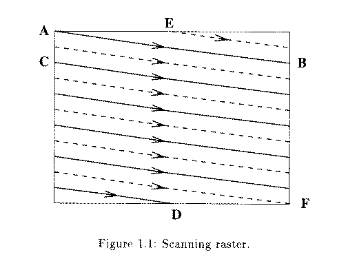
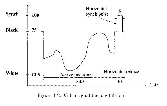
- Each line takes 63.5 microseconds to scan. Horizontal retrace takes 10 microseconds (with 5 microseconds horizontal synch pulse embedded), so the active line time is 53.5 microseconds.
- Color representation:
- NTSC uses YIQ color model.
- composite = Y + I cos(Fsc t) + Q sin(Fsc t), where Fsc is the frequency of color subcarrier
Digital Video Rasters
PAL Video
- 625 scan lines per frame, 25 frames per second (40 msec/frame)
- Interlaced, each frame is divided into 2 fields, 312.5 lines/field
- Uses YUV color model
Digital Video
- Advantages:
- Direct random access --> good for nonlinear video editing
- No problem for repeated recording
- No need for blanking and sync pulse
- Almost all digital video uses component video
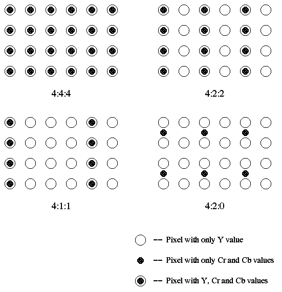
Chroma Subsampling
- How to decimate for chrominance?
- 4:4:4 --> No chroma subsampling, each pixel has Y, Cr and Cb values.
- 4:1:1 and 4:2:0 are mostly used in JPEG and MPEG (see Chapter 4).
4:2:2 --> Horizontally subsample Cr, Cb signals by a factor of 2.
4:1:1 --> Horizontally subsampled by a factor of 4.
4:2:0 --> Subsampled in both the horizontal and vertical dimensions by a factor of 2. Theoretically, the chroma pixel is positioned between the rows and columns as shown in the figure.
CCIR Standards for Digital Video
(CCIR -- Consultative Committee for International Radio)CCIR 601 CCIR 601 CIF QCIF 525/60 625/50 NTSC PAL/SECAM -------------------- ----------- ----------- ----------- ----------- Luminance resolution 720 x 485 720 x 576 352 x 288 176 x 144 Chrominance resolut. 360 x 485 360 x 576 176 x 144 88 x 72 Color Subsampling 4:2:2 4:2:2 4:2:0 4:2:0 Fields/sec 60 50 30 30 Interlacing Yes Yes No No
- CCIR 601 uses interlaced scan, so each field only has half as much vertical resolution (e.g., 243 lines in NTSC). The CCIR 601 (NTSC) data rate is ~165 Mbps.
- CIF (Common Intermediate Format) -- an acceptable temporary standard
- Approximately the VHS quality
- Uses progressive (non-interlaced) scan
- Uses NTSC frame rate, and half the active lines of PAL signals --> To play on existing TVs, PAL systems need to do frame rate conversion, and NTSC systems need to do line-number conversion.
- QCIF -- Quarter-CIF
ATSC Digital Television Standard
(ATSC -- Advanced Television Systems Committee) The ATSC Digital Television Standard was recommended to be adopted as the Advanced TV broadcasting standard by the FCC Advisory Committee on Advanced Television Service on November 28, 1995. It covers the standard for HDTV (High Definition TV). Video FormatThe video scanning formats supported by the ATSC Digital Television Standard are shown in the following table.
- The aspect ratio for HDTV is 16:9 as opposed to 4:3 in NTSC, PAL, and SECAM. (A 33% increase in horizontal dimension.)
- In the picture rate column, the "I" means interlaced scan, and the "P" means progressive (non-interlaced) scan.
- Both NTSC rates and integer rates are supported (i.e., 60.00, 59.94, 30.00, 29.97, 24.00, and 23.98).
- At 1920 x 1080, 60I (which CBS and NBC have selected), there will be 1920 x 1080 x 30 = 62.2 millions pixels per second. Considering 4:2:2 chroma subsampling, each pixel needs 16 bits to represent, the bit rate is 62.2 x 16 = 995 Mb/sec.
book
http://eeweb.poly.edu/~yao/videobook/
Introduction
The purpose of this lab is to acquaint you with the TI Image Developers Kit (IDK). The IDK contains a floating point C6711 DSP, and other hardware that enables real time video/image processing. In addition to the IDK, the video processing lab bench is equipped with an NTSC camera and a standard color computer monitor.
You will complete an introductory exercise to gain familiarity with the IDK programming environment. In the exercise, you will modify a C skeleton to horizontally flip and invert video input (black and white) from the camera. The output of your video processing algorithm will appear in the top right quadrant of the monitor.
In addition, you will analyze existing C code that implements filtering and edge detection algorithms to gain insight into IDK programming methods. The output of these "canned" algorithms, along with the unprocessed input, appears in the other quadrants of the monitor.
Finally, you will create an auto contrast function. And will also work with a color video feed and create a basic user interface, which uses the input to control some aspect of the display.
An additional goal of this lab is to give you the opportunity to discover tools for developing an original project using the IDK.
Important Documentation
The following documentation will certainly prove useful:
The IDK
User's Guide. Section 2 is the most important. The IDK
Video Device Drivers User's Guide. The sections on timing are not too important, but pay attention to the Display and Capture systems and have a good idea of how they work. The IDK
Programmer's Guide. Sections 2 and 5 are the ones needed. Section 2 is very, very important in Project Lab 2. It is also useful in understanding “streams” in project lab 1.
Note: Other manuals may be found on TI's website by searching for
TMS320C6000 IDK
Video Processing - The Basics
The camera on the video processing lab bench generates a video signal in NTSC format. NTSC is a standard for transmitting and displaying video that is used in television. The signal from the camera is connected to the "composite input" on the IDK board (the yellow plug). This is illustrated in Figure 2-1 on page 2-3 of the IDK User's Guide. Notice that the IDK board is actually two boards stacked on top of each other. The bottom board contains the C6711 DSP, where your image processing algorithms will run. The daughterboard is on top, it contains the hardware for interfacing with the camera input and monitor output. For future video processing projects, you may connect a video input other than the camera, such as the output from a DVD player. The output signal from the IDK is in RGB format, so that it may be displayed on a computer monitor.
At this point, a description of the essential terminology of the IDK environment is in order. The video input is first decoded and then sent to the FPGA, which resides on the daughterboard. The FPGA is responsible for video capture and for the filling of the input frame buffer (whose contents we will read). For a detailed description of the FPGA and its functionality, we advise you to read Chapter 2 of the IDK User's Guide.
The Chip Support Library (CSL) is an abstraction layer that allows the IDK daughterboard to be used with the entire family of TI C6000 DSPs (not just the C6711 that we're using); it takes care of what is different from chip to chip.
The Image Data Manager (IDM) is a set of routines responsible for moving data between on-chip internal memory, and external memory on the board, during processing. The IDM helps the programmer by taking care of the pointer updates and buffer management involved in transferring data. Your DSP algorithms will read and write to internal memory, and the IDM will transfer this data to and from external memory. Examples of external memory include temporary "scratch pad" buffers, the input buffer containing data from the camera, and the output buffer with data destined for the RGB output.
The two different memory units exist to provide rapid access to a larger memory capacity. The external memory is very large in size – around 16 MB, but is slow to access. But the internal is only about 25 KB or so and offers very fast access times. Thus we often store large pieces of data, such as the entire input frame, in the external memory. We then bring it in to internal memory, one small portion at a time, as needed. A portion could be a line or part of a line of the frame. We then process the data in internal memory and then repeat in reverse, by outputting the results line by line (or part of) to external memory. This is full explained in Project Lab 2, and this manipulation of memory is important in designing efficient systems.
The TI C6711 DSP uses a different instruction set than the 5400 DSP's you are familiar with in lab. The IDK environment was designed with high level programming in mind, so that programmers would be isolated from the intricacies of assembly programming. Therefore, we strongly suggest that you do all your programming in C. Programs on the IDK typically consist of a main program that calls an image processing routine.
The main program serves to setup the memory spaces needed and store the pointers to these in objects for easy access. It also sets up the input and output channels and the hardware modes (color/grayscale ...). In short it prepares the system for our image processing algorithm.
The image processing routine may make several calls to specialized functions. These specialized functions consist of an outer wrapper and an inner component. The wrapper oversees the processing of the entire image, while the component function works on parts of an image at a time. And the IDM moves data back and forth between internal and external memory.
As it brings in one line in from external memory, the component function performs the processing on this one line. Results are sent back to the wrapper. And finally the wrapper contains the IDM instructions to pass the output to external memory or wherever else it may be needed.
Please note that this is a good methodology used in programming for the IDK. However it is very flexible too, the "wrapper" and "component functions" are C functions and return values, take in parameters and so on too. And it is possible to extract/output multiple lines or block etc. as later shown.
In this lab, you will modify a component to implement the flipping and inverting algorithm. And you will perform some simple auto-contrasting as well as work with color.
In addition, the version of Code Composer that the IDK uses is different from the one you have used previously. The IDK uses Code Composer Studio v2.1. It is similar to the other version, but the process of loading code is slightly different.
Code DescriptionOverview and I/O
The next few sections describe the code used. First please copy the files needed by following the instructions in the "Part 1" section of this document. This will help you easily follow the next few parts.
The program flow for image processing applications may be a bit different from your previous experiences in C programming. In most C programs, the main function is where program execution starts and ends. In this real-time application, the main function serves only to setup initializations for the cache, the CSL, and the DMA (memory access) channel. When it exits, the main task, tskMainFunc(), will execute automatically, starting the DSP/BIOS. It will loop continuously calling functions to operate on new frames and this is where our image processing application begins.
The tskMainFunc(), in main.c, opens the handles to the board for image capture (VCAP_open()) and to the display (VCAP_open()) and calls the grayscale function. Here, several data structures are instantiated that are defined in the file img_proc.h. The IMAGE structures will point to the data that is captured by the FPGA and the data that will be output to the display. The SCRATCH_PAD structure points to our internal and external memory buffers used for temporary storage during processing. LPF_PARAMS is used to store filter coefficients for the low pass filter.
The call to img_proc() takes us to the file img_proc.c. First, several variables are declared and defined. The variable quadrant will denote on which quadrant of the screen we currently want output; out_ptr will point to the current output spot in the output image; and pitch refers to the byte offset (distance) between two lines. This function is the high level control for our image-processing algorithm. See algorithm flow.
Figure 1: Algorithm FlowFigure 1 (video1.jpg)
The first function called is the pre_scale_image function in the file pre_scale_image.c. The purpose of this function is to take the 640x480 image and scale it down to a quarter of its size by first downsampling the input rows by two and then averaging every two pixels horizontally. The internal and external memory spaces, pointers to which are in the scratch pad, are used for this task. The vertical downsampling occurs when every other line is read into the internal memory from the input image. Within internal memory, we will operate on two lines of data (640 columns/line) at a time, averaging every two pixels (horizontal neighbors) and producing two lines of output (320 columns/line) that are stored in the external memory.
To accomplish this, we will need to take advantage of the IDM by initializing the input and output streams. At the start of the function, two instantiations of a new structure dstr_t are declared. You can view the structure contents of dstr_t on p. 2-11 of the IDK Programmer's Guide. These structures are stream "objects". They give us access to the data when using the dstr_open() command. In this case dstr_i is an input stream as specified in the really long command dstr_open(). Thus after opening this stream we can use the get_data command to get data one line at a time. Streams and memory usage are described in greater detail in the second project lab. This data flow for the pre-scale is shown in data flow.
Figure 2: Data flow of input and output streams.Figure 2 (video2.jpg)
To give you a better understanding of how these streams are created, let's analyze the parameters passed in the first call to dstr_open() which opens an input stream.
External address: in_image->data
This is a pointer to the place in external memory serving as the source of our input data (it's the source because the last function parameter is set to DSTR_INPUT). We're going to bring in data from external to internal memory so that we can work on it. This external data represents a frame of camera input. It was captured in the main function using the VCAP_getframe() command.
External size: (rows + num_lines) * cols = (240 + 2) * 640
This is the total size of the input data which we will bring in. We will only be taking two lines at a time from in_image->data, so only 240 rows. The "plus 2" represents two extra rows of input data which represent a buffer of two lines - used when filtering, which is explained later.
Internal address: int_mem
This is a pointer to an 8x640 array, pointed to by scratchpad->int_data. This is where we will be putting the data on each call to dstr_get(). We only need part of it, as seen in the next parameter, as space to bring in data.
Internal size: 2 * num_lines * cols = 2 * 2 * 640
The size of space available for data to be input into int_mem from in_image->data. We pull in two lines of the input frame so it num_lines * cols. We have the multiply by 2 as we are using double buffering for bringing in the data. We need double the space in internal memory than the minimum needed, the reason is fully explained in IDK Programmer's Guide.
Number of bytes/line: cols = 640, Number of lines: num_lines = 2
Each time dstr_get_2D() is called, it will return a pointer to 2 new lines of data, 640 bytes in length. We use the function dstr_get_2D(), since we are pulling in two lines of data. If instead we were only bringing in one line, we would use dstr_get() statements.
External memory increment/line: stride*cols = 1*640
The IDM increments the pointer to the external memory by this amount after each dstr_get() call.
Window size: 1 for double buffered single line of data
(Look at the three documentation pdfs for a full explanation of double buffering)
The need for the window size is not really apparent here.
It will become apparent when we do the 3x3 block convolution. Then, the window size will be set to 3 (indicating three lines of buffered data). This tells the IDM to send a pointer to extract 3 lines of data when dstr_get() is called, but only increment the stream's internal pointer by 1 (instead of 3) the next time dstr_get() is called. Thus you will get overlapping sets of 3 lines on each dstr_get() call. This is not a useful parameter when setting up an output stream.
Direction of input: DSTR_INPUT
Sets the direction of data flow. If it had been set to DSTR_OUTPUT (as done in the next call to dstr_open()), we would be setting the data to flow from the Internal Address to the External Address.
We then setup our output stream to write data to a location in external memory which we had previously created.
Once our data streams are setup, we can begin processing by first extracting a portion of input data using dstr_get_2D(). This command pulls the data in and we setup a pointer (in_data) to point to this internal memory spot. We also get a pointer to a space where we can write the output data (out_data) when using dstr_put(). Then we call the component function pre_scale() (in pre_scale.c) to operate on the input data and write to the output data space, using these pointers.
The prescaling function will perform the horizontal scaling by averaging every two pixels. This algorithm operates on four pixels at a time. The entire function is iterated within pre_scale_image() 240 times, which results in 240 * 2 rows of data being processed – but only half of that is output.
Upon returning to the wrapper function, pre_scale_image, a new line is extracted; the pointers are updated to show the location of the new lines and the output we had placed in internal memory is then transferred out. This actually happens in the dstr_put() function – thus is serves a dual purpose; to give us a pointer to internal memory which we can write to, and the transferring of its contents to external memory.
Before pre_scale_image() exits, the data streams are closed, and one line is added to the top and bottom of the image to provide context necessary for the next processing steps (The extra two lines - remember?). Also note, it is VERY important to close streams after they have been used.
If not done, unusual things such as random crashing and so may occur which are very hard to track down.
Now that the input image has been scaled to a quarter of its initial size, we will proceed with the four image processing algorithms. In img_proc.c, the set_ptr() function is called to set the variable out_ptr to point to the correct quadrant on the 640x480 output image. Then copy_image(), copy_image.c, is called, performing a direct copy of the scaled input image into the lower right quadrant of the output.
Next we will set the out_ptr to point to the upper right quadrant of the output image and call conv3x3_image() in conv3x3_image.c. As with pre_scale_image(), the _image indicates this is only the wrapper function for the ImageLIB (library functions) component, conv3x3(). As before, we must setup our input and output streams. This time, however, data will be read from the external memory (where we have the pre-scaled image) and into internal memory for processing, and then be written to the output image. Iterating over each row, we compute one line of data by calling the component function conv3x3() in conv3x3.c.
In conv3x3(), you will see that we perform a 3x3 block convolution, computing one line of data with the low pass filter mask. Note here that the variables IN1[i], IN2[i], and IN3[i] all grab only one pixel at a time. This is in contrast to the operation of pre_scale() where the variable in_ptr[i] grabbed 4 pixels at a time. This is because in_ptr was of type unsigned int, which implies that it points to four bytes (the size of an unsigned int is 4 bytes) of data at a time. IN1, IN2, and IN3 are all of type unsigned char, which implies they point to a single byte of data. In block convolution, we are computing the value of one pixel by placing weights on a 3x3 block of pixels in the input image and computing the sum. What happens when we are trying to compute the rightmost pixel in a row? The computation is now bogus. That is why the wrapper function copies the last good column of data into the two rightmost columns. You should also note that the component function ensures output pixels will lie between 0 and 255. For the same reason we provided the two extra "copied" lines when performing the prescale.
Back in img_proc.c, we can begin the edge detection algorithm, sobel_image(), for the lower left quadrant of the output image. This wrapper function, located in sobel_image.c, performs edge detection by utilizing the assembly written component function sobel() in sobel.asm. The wrapper function is very similar to the others you have seen and should be straightforward to understand. Understanding the assembly file is considerably more difficult since you are not familiar with the assembly language for the c6711 DSP. As you'll see in the assembly file, the comments are very helpful since an "equivalent" C program is given there.
The Sobel algorithm convolves two masks with a 3x3 block of data and sums the results to produce a single pixel of output. One mask has a preference for vertical edges while the other mask for horizontal ones. This algorithm approximates a 3x3 nonlinear edge enhancement operator. The brightest edges in the result represent a rapid transition (well-defined features), and darker edges represent smoother transitions (blurred or blended features).
Part One
This section provides a hands-on introduction to the IDK environment that will prepare you for the lab exercise. First, connect the power supply to the IDK module. Two green lights on the IDK board should be illuminated when the power is connected properly.
You will need to create a directory img_proc for this project in your home directory. Enter this new directory, and then copy the following files as follows (again, be sure you're in the directory img_proc when you do this):
copy V:\ece320\idk\c6000\IDK\Examples\NTSC\img_proc copy V:\ece320\idk\c6000\IDK\Drivers\include copy V:\ece320\idk\c6000\IDK\Drivers\lib
After the IDK is powered on, open Code Composer 2 by clicking on the "CCS 2" icon on the desktop. From the "Project" menu, select "Open," and then open img_proc.pjt. You should see a new icon appear at the menu on the left side of the Code Composer window with the label img_proc.pjt. Double click on this icon to see a list of folders. There should be a folder labeled "Source." Open this folder to see a list of program files.
The main.c program calls the img_proc.c function that displays the output of four image processing routines in four quadrants on the monitor. The other files are associated with the four image processing routines. If you open the "Include" folder, you will see a list of header files. To inspect the main program, double click on the main.c icon. A window with the C code will appear to the right.
Scroll down to the tskMainFunc() in the main.c code. A few lines into this function, you will see the line LOG_printf(&trace,"Hello\n"). This line prints a message to the message log, which can be useful for debugging. Change the message "Hello\n" to "Your Name\n" (the "\n" is a carriage return). Save the file by clicking the little floppy disk icon at the top left corner of the Code Composer window.
To compile all of the files when the ".out" file has not yet been generated, you need to use the "Rebuild All" command. The rebuild all command is accomplished by clicking the button displaying three little red arrows pointing down on a rectangular box. This will compile every file the main.c program uses. If you've only changed one file, you only need to do a "Incremental Build," which is accomplished by clicking on the button with two little blue arrows pointing into a box (immediately to the left of the "Rebuild All" button). Click the "Rebuild All" button to compile all of the code. A window at the bottom of Code Composer will tell you the status of the compiling (i.e., whether there were any errors or warnings). You might notice some warnings after compilation - don't worry about these.
Click on the "DSP/BIOS" menu, and select "Message Log." A new window should appear at the bottom of Code Composer. Assuming the code has compiled correctly, select "File" -> "Load Program" and load img_proc.out (the same procedure as on the other version of Code Composer). Now select "Debug" -> "Run" to run the program (if you have problems, you may need to select "Debug" -> "Go Main" before running). You should see image processing routines running on the four quadrants of the monitor. The upper left quadrant (quadrant 0) displays a low pass filtered version of the input. The low pass filter "passes" the detail in the image, and attenuates the smooth features, resulting in a "grainy" image. The operation of the low pass filter code, and how data is moved to and from the filtering routine, was described in detail in the previous section. The lower left quadrant (quadrant 2) displays the output of an edge detection algorithm. The top right and bottom right quadrants (quadrants 1 and 3, respectively), show the original input displayed unprocessed. At this point, you should notice your name displayed in the message log.
Friday, May 25, 2012
kile in windows
http://sourceforge.net/apps/mediawiki/kile/index.php?title=KileOnWindows
http://www.latex-community.org/forum/viewtopic.php?f=20&t=1563
http://en.wikipedia.org/wiki/Comparison_of_TeX_editors
http://www.winedt.com/download.html
http://www.winshell.org/modules/ws_screenshots/
http://tug.org/pracjourn/2008-1/mori/mori.pdf
http://www.latex-community.org/forum/viewtopic.php?f=20&t=1563
http://en.wikipedia.org/wiki/Comparison_of_TeX_editors
http://www.winedt.com/download.html
http://www.winshell.org/modules/ws_screenshots/
http://tug.org/pracjourn/2008-1/mori/mori.pdf
Sunday, May 13, 2012
Happy mothers day.......The Mother monkey and her baby
The Mother monkey and her baby

A baby monkey was injured while crossing the busy street. The Mother monkey charged on vehicles and attacked a stray dog to save her baby in Jaipur.

A baby monkey was injured while crossing the busy street. The Mother monkey charged on vehicles and attacked a stray dog to save her baby in Jaipur.

A baby monkey was injured while crossing the busy street. The Mother monkey charged on vehicles and attacked a stray dog to save her baby in Jaipur.

A baby monkey was injured while crossing the busy street. The Mother monkey charged on vehicles and attacked a stray dog to save her baby in Jaipur.

A baby monkey was injured while crossing the busy street. The Mother monkey charged on vehicles and attacked a stray dog to save her baby in Jaipur.

A baby monkey was injured while crossing the busy street. The Mother monkey charged on vehicles and attacked a stray dog to save her baby in Jaipur.
Thursday, May 10, 2012
Institute Valedictory Function Class of 2012 by Speaker: Dr. D. B. Phatak
Link : http://www.youtube.com/watch?v=eUebtM-uS3w
Speaker: Dr. D. B. Phatak, Subrao Nilekani Chair Professor, Department of Computer Science and Engineering, IIT Bombay Listed amongst fifty most influential Indians by Business week 2009
Prof Phatak giving the sending-off lecture to the graduating class of 2012 themed on "Building India Where Dreams Come True - Journey to an exciting professional career" at IIT Bombay, Mumbai, 3rd May, 2012.
Called the Institute Valedictory Function, the event was very well received by a jam-packed audience at the VMCC auditorium, with students taking back a great sense of pride and honour as graduates from IITB, with a sense of giving back to the institution, which makes them what they are today, and what they will be tomorrow.
For all updates related to the Student Alumni Relations Cell, subscribe to our channel and visit http://sarc-iitb.org/
Wednesday, May 9, 2012
Y'UV422 , RGB888 Formats
Y'UV422 to RGB888 conversion
http://en.wikipedia.org/wiki/YUVY'UV422 to RGB888 conversion
- Input: Read 4 bytes of Y'UV (u, y1, v, y2 )
- Output: Writes 6 bytes of RGB (R, G, B, R, G, B)
y1 = yuv[0];
u  = yuv[1];
y2 = yuv[2];
v  = yuv[3];
Using this information it could be parsed as regular Y'UV444 format to get 2 RGB pixels info:
rgb1 = Y'UV444toRGB888(y1, u, v);
rgb2 = Y'UV444toRGB888(y2, u, v);
Y'UV422 can also be expressed in YUY2 FourCC format code. That means 2 pixels will be defined in each macropixel (four bytes) treated in the image.
 .
.Y'UV411 to RGB888 conversion
- Input: Read 6 bytes of Y'UV
- Output: Writes 12 bytes of RGB
// Extract YUV components
u  = yuv[0];
y1 = yuv[1];
y2 = yuv[2];
v  = yuv[3];
y3 = yuv[4];
y4 = yuv[5];
rgb1 = Y'UV444toRGB888(y1, u, v);
rgb2 = Y'UV444toRGB888(y2, u, v);
rgb3 = Y'UV444toRGB888(y3, u, v);
rgb4 = Y'UV444toRGB888(y4, u, v);
So the result is we are getting 4 RGB pixels values (4*3 bytes) from 6 bytes. This means reducing the size of transferred data to half, with a loss of quality.
Y'UV420p (and Y'V12 or YV12) to RGB888 conversion
Y'UV420p is a planar format, meaning that the Y', U, and V values are grouped together instead of interspersed. The reason for this is that by grouping the U and V values together, the image becomes much more compressible. When given an array of an image in the Y'UV420p format, all the Y' values come first, followed by all the U values, followed finally by all the V values.The Y'V12 format is essentially the same as Y'UV420p, but it has the U and V data switched: the Y' values are followed by the V values, with the U values last. As long as care is taken to extract U and V values from the proper locations, both Y'UV420p and Y'V12 can be processed using the same algorithm.
As with most Y'UV formats, there are as many Y' values as there are pixels. Where X equals the height multiplied by the width, the first X indices in the array are Y' values that correspond to each individual pixel. However, there are only one fourth as many U and V values. The U and V values correspond to each 2 by 2 block of the image, meaning each U and V entry applies to four pixels. After the Y' values, the next X/4 indices are the U values for each 2 by 2 block, and the next X/4 indices after that are the V values that also apply to each 2 by 2 block.
Translating Y'UV420p to RGB is a more involved process compared to the previous formats. Lookup of the Y', U and V values can be done using the following method:
size.total = size.width * size.height;
y = yuv[position.y * size.width + position.x];
u = yuv[(position.y / 2) * (size.width / 2) + (position.x / 2) + size.total];
v = yuv[(position.y / 2) * (size.width / 2) + (position.x / 2) + size.total + (size.total / 4)];
rgb = Y'UV444toRGB888(y, u, v);
Here "/" is Div not division.

As shown in the above image, the Y', U and V components in Y'UV420 are encoded separately in sequential blocks. A Y' value is stored for every pixel, followed by a U value for each 2×2 square block of pixels, and finally a V value for each 2×2 block. Corresponding Y', U and V values are shown using the same color in the diagram above. Read line-by-line as a byte stream from a device, the Y' block would be found at position 0, the U block at position x×y (6×4 = 24 in this example) and the V block at position x×y + (x×y)/4 (here, 6×4 + (6×4)/4 = 30).
http://en.wikipedia.org/wiki/YCbCr
http://www.mathworks.com/matlabcentral/fileexchange/31625-convert-rgb-to-yuv/content/convert_RGB_to_YUV.m
http://www.fourcc.org/fccyvrgb.php
http://stackoverflow.com/questions/1945374/convert-yuv-sequence-to-bmp-images
rgb = imread('board.tif');
ycbcr = rgb2ycbcr(rgb);
rgb2 = ycbcr2rgb(ycbcr);
http://amath.colorado.edu/computing/Matlab/Tutorial/ImageProcess.html
Selecting Rows and Columns of a Matrix
http://langvillea.people.cofc.edu/DISSECTION-LAB/Emmie%27sBibleCodeModule/matlabtutorial.html
Tuesday, May 8, 2012
matlab read and write to file
how to write data into a file
_________________________________csvwrite('attr20.ascii',A); csvwrite(filename,M) csvwrite(filename,M,row,col)
--------------------dlmwrite(filename, M) dlmwrite(filename, M, 'D') dlmwrite(filename, M, 'D', R, C)
dlmwrite('myfile.txt', M, 'delimiter', '\t', ...
         'precision', 6)
type myfile.txt
0.893898      0.284409      0.582792      0.432907
0.199138      0.469224      0.423496      0.22595
0.298723      0.0647811     0.515512      0.579807
0.661443      0.988335      0.333951      0.760365
http://www.mathworks.in/help/techdoc/ref/dlmwrite.html
http://www.myoutsourcedbrain.com/2008/11/export-data-from-matlab.html
http://www.mathworks.com/matlabcentral/newsreader/view_thread/314766
http://www.mathworks.com/matlabcentral/newsreader/view_thread/314766
--------------------------------
Write dataset array to file
Syntax
export(DS,'file',filename)export(DS)
export(DS,'file',filename,'Delimiter',delim)
read to file M = csvread(filename) M = csvread(filename, row, col)
http://www.mathworks.in/help/techdoc/ref/csvread.html
more info type 'csvread' in matlab help
-------------------------
A = fread(fileID)
A = fread(fileID, sizeA)
---------------
[A,B,C,...] = textread(filename,format)
------------- http://www.mathworks.in/help/matlab/import_export/supported-file-formats.html
------http://ocw.mit.edu/resources/res-18-002-introduction-to-matlab-spring-2008/other-matlab-resources-at-mit/tutorial05.pdf
FOR LOOPhttp://www.cyclismo.org/tutorial/matlab/control.htmlhttp://www.math.utah.edu/~wright/misc/matlab/programmingintro.htmlhttp://www.cs.utah.edu/~germain/PPS/Topics/Matlab/plot.html
sub plot subplot(1,2,1), imshow('autumn.tif');
subplot(1,2,2), imshow('glass.png');
Function
function [out1, out2, ...] = myfun(in1,in2, ...)
Example
function [mean,stdev] = stat(x)
n = length(x);
mean = sum(x)/n;
stdev = sqrt(sum((x-mean).^2/n));
Subscribe to:
Posts (Atom)