latex_equation,table_symble help

 

Ref: http://en.wikibooks.org/wiki/LaTeX/Mathematics 

http://crab.rutgers.edu/~karel/latex/class4/class4.html

LaTeX/Mathematics

< LaTeX

The latest reviewed version was checked on 30 April 2012. There are 5 pending changes awaiting review.

Jump to: navigation, search

LaTeX

One of the greatest motivating forces for Donald Knuth when he began developing the original TeX system was to create something that allowed simple construction of mathematical formulas, whilst looking professional when printed. The fact that he succeeded was most probably why TeX (and later on, LaTeX) became so popular within the scientific community. Typesetting mathematics is one of LaTeX's greatest strengths. It is also a large topic due to the existence of so much mathematical notation.
If your document requires only a few simple mathematical formulas, plain LaTeX has most of the tools that you will need. If you are writing a scientific document that contains numerous complicated formulas, the amsmath package^[1] introduces several new commands that are more powerful and flexible than the ones provided by LaTeX. The mathtools package fixes some amsmath quirks and adds some useful settings, symbols, and environments to amsmath.^[2] To use either package, include:

\usepackage{amsmath}

or

\usepackage{mathtools}

in the preamble of the document. The mathtools package loads the amsmath package and hence there is no need to \usepackage{amsmath} in the preamble if mathtools is used.

Contents 1 Mathematics environments 1.1 Inserting "Displayed" maths inside blocks of text 2 Symbols 3 Greek letters 4 Operators 5 Powers and indices 6 Fractions and Binomials 6.1 Continued fractions 6.2 Multiplication of two numbers 7 Roots 8 Sums and integrals 9 Brackets, braces and delimiters 9.1 Automatic sizing 9.2 Manual sizing 10 Matrices and arrays 10.1 Matrices in running text 11 Adding text to equations 11.1 Formatted text 12 Formatting mathematics symbols 12.1 Accents 13 Plus and minus signs 14 Controlling horizontal spacing 15 Advanced Mathematics: AMS Math package 15.1 Introducing text and dots in formulas 15.2 Dots 16 List of Mathematical Symbols 17 Summary 18 Notes 19 Further reading 20 External links

Mathematics environments

LaTeX needs to know beforehand that the subsequent text does in fact contain mathematical elements. This is because LaTeX typesets maths notation differently than normal text. Therefore, special environments have been declared for this purpose. They can be distinguished into two categories depending on how they are presented:

• text - text formulas are displayed in-line, that is, within the body of text where it is declared. e.g., I can say that a + a = 2a within this sentence.
• displayed - displayed formulas are separate from the main text.

As maths require special environments, there are naturally the appropriate environment names you can use in the standard way. Unlike most other environments, however, there are some handy shorthands to declaring your formulas. The following table summarizes them:

Type	Environment	LaTeX shorthand	TeX shorthand
Text	\begin{math}...\end{math}	\(...\)	$...$
Displayed	\begin{displaymath}...\end{displaymath} or \begin{equation*}...\end{equation*}[3]	\[...\]	$$...$$

Note: Using the $$...$$ should be avoided, as it may cause problems, particularly with the AMS-LaTeX macros. Furthermore, should a problem occur, the error messages may not be helpful.
Additionally, there is a second possible environment for the displayed type of formulas: equation. The difference between this and displaymath is that equation also adds sequential equation numbers by the side.
If you are typing text normally, you are said to be in text mode, while you are typing within one of those mathematical environments, you are said to be in math mode, that has some differences compared to the text mode:

1. Most spaces and line breaks do not have any significance, as all spaces are either derived logically from the mathematical expressions, or have to be specified with special commands such as \quad
2. Empty lines are not allowed. Only one paragraph per formula.
3. Each letter is considered to be the name of a variable and will be typeset as such. If you want to typeset normal text within a formula (normal upright font and normal spacing) then you have to enter the text using dedicated commands.

Inserting "Displayed" maths inside blocks of text

In order for some operators, such as \lim or \sum to be displayed correctly inside some math environments (read $......$), it might be convenient to write the \displaystyle class inside the environment. Doing so might cause the line to be taller, but will cause exponents and indices to be displayed correctly for some math operators. For example, the $\sum$ will print a smaller Σ and $\displaystyle \sum$ will print a bigger one , like in equations (This only works with AMSMATH package).

Symbols

Mathematics has lots and lots of symbols! If there is one aspect of maths that is difficult in LaTeX it is trying to remember how to produce them. There are of course a set of symbols that can be accessed directly from the keyboard:

+ - = ! / ( ) [ ] < > | ' :

Beyond those listed above, distinct commands must be issued in order to display the desired symbols. And there are a lot! of Greek letters, set and relations symbols, arrows, binary operators, etc. For example:

\[  \forall x \in X, \quad \exists y \leq \epsilon \]

Fortunately, there's a tool that can greatly simplify the search for the command for a specific symbol. Look for "Detexify" in the external links section below. Another option would be to look in the "The Comprehensive LaTeX Symbol List" in the external links section below.

Greek letters

Greek letters are commonly used in mathematics, and they are very easy to type in math mode. You just have to type the name of the letter after a backslash: if the first letter is lowercase, you will get a lowercase Greek letter, if the first letter is uppercase (and only the first letter), then you will get an uppercase letter. Note that some uppercase Greek letters look like Latin ones, so they are not provided by LaTeX (e.g. uppercase Alpha and Beta are just "A" and "B" respectively). Lowercase epsilon, theta, phi, pi, rho, and sigma are provided in two different versions. The alternate, or variant, version is created by adding "var" before the name of the letter:

\[   \alpha, \Alpha, \beta, \Beta, \gamma, \Gamma,   \pi, \Pi, \phi, \varphi, \Phi \]

Scroll down to #List of Mathematical Symbols for a complete list of Greek symbols.

Operators

An operator is a function that is written as a word: e.g. trigonometric functions (sin, cos, tan), logarithms and exponentials (log, exp). LaTeX has many of these defined as commands:

\[  \cos (2\theta) = \cos^2 \theta - \sin^2 \theta \]

For certain operators such as limits, the subscript is placed underneath the operator:

\[  \lim_{x \to \infty} \exp(-x) = 0 \]

For the modular operator there are two commands: \bmod and \pmod:

\[  a \bmod b \]

\[  x \equiv a \pmod b \]

To use operators which are not pre-defined, such as argmax, see custom operators

Powers and indices

Powers and indices are equivalent to superscripts and subscripts in normal text mode. The caret (^) character is used to raise something, and the underscore (_) is for lowering. If more than one expression is raised or lowered, they should be grouped using curly braces ({ and }).

\[  k_{n+1} = n^2 + k_n^2 - k_{n-1} \]

An underscore (_) can be used with a vertical bar () to denote evaluation using subscript notation in mathematics:

\[  f(n) = n^5 + 4n^2 + 2 |_{n=17} \]

Fractions and Binomials

A fraction is created using the \frac{numerator}{denominator} command. (for those who need their memories refreshed, that's the top and bottom respectively!). Likewise, the binomial coefficient (aka the Choose function) may be written using the \binom command^[3]:

\[  \frac{n!}{k!(n-k)!} = \binom{n}{k} \]

It is also possible to use the \choose command without the amsmath package:

\[  \frac{n!}{k!(n-k)!} = {n \choose k} \]

You can embed fractions within fractions:

\[  \frac{\frac{1}{x}+\frac{1}{y}}{y-z} \]

Note that when appearing inside another fraction, or in inline text , a fraction is noticeably smaller than in displayed mathematics. The \tfrac and \dfrac commands^[3] force the use of the respective styles, \textstyle and \displaystyle. Similarly, the \tbinom and \dbinom commands typeset the binomial coefficient.
Another way to write fractions is to use the \over command without the amsmath package:

\[  {n! \over k!(n-k)!} = {n \choose k} \]

For relatively simple fractions, it may be more aesthetically pleasing to use powers and indices:

\[  ^3/_7 \]

If you use them throughout the document, usage of xfrac package is recommended. This package provides \sfrac command to create slanted fractions. Usage:

Take \sfrac{1}{2} cup of sugar, \dots  \[   3\times\sfrac{1}{2}=1\sfrac{1}{2}  \] Take ${}^1/_2$ cup of sugar, \dots  \[   3\times{}^1/_2=1{}^1/_2  \]

Alternatively, the nicefrac package provides the \nicefrac command, whose usage is similar to \sfrac.

Continued fractions

Continued fractions should be written using \cfrac command^[3]:

\begin{equation}   x = a_0 + \cfrac{1}{a_1           + \cfrac{1}{a_2           + \cfrac{1}{a_3 + a_4}}}\end{equation}

Multiplication of two numbers

To make multiplication visually similar to a fraction, a nested array can be used, for example multiplication of numbers written one below the other.

\begin{equation} \frac{     \begin{array}[b]{r}       \left( x_1 x_2 \right)\\       \times \left( x'_1 x'_2 \right)     \end{array}   }{     \left( y_1y_2y_3y_4 \right)   }\end{equation}

Roots

The \sqrt command creates a square root surrounding an expression. It accepts an optional argument specified in square brackets ([ and ]) to change magnitude:

\[ \sqrt{\frac{a}{b}} \]

\[ \sqrt[n]{1+x+x^2+x^3+\ldots} \]

Some people prefer writing the square root "closing" it over its content. This method arguably makes it more clear what is in the scope of the root sign. This habit is not normally used while writing with the computer, but if you still want to change the output of the square root, LaTeX gives you this possibility. Just add the following code in the preamble of your document:

% New definition of square root: % it renames \sqrt as \oldsqrt \let\oldsqrt\sqrt % it defines the new \sqrt in terms of the old one \def\sqrt{\mathpalette\DHLhksqrt} \def\DHLhksqrt#1#2{% \setbox0=\hbox{$#1\oldsqrt{#2\,}$}\dimen0=\ht0 \advance\dimen0-0.2\ht0 \setbox2=\hbox{\vrule height\ht0 depth -\dimen0}% {\box0\lower0.4pt\box2}}

The new style is on left, the old one on right

This TeX code first renames the \sqrt command as \oldsqrt, then redefines \sqrt in terms of the old one, adding something more. The new square root can be seen in the picture on the left, compared to the old one on the right. Unfortunately this code won't work if you want to use multiple roots: if you try to write as \sqrt[b]{a} after you used the code above, you'll just get a wrong output. In other words, you can redefine the square root this way only if you are not going to use multiple roots in the whole document.
An alternative piece of TeX code that does allow multiple roots is

\LetLtxMacro{\oldsqrt}{\sqrt} % makes all sqrts closed \renewcommand{\sqrt}[1][]{%   \def\DHLindex{#1}\mathpalette\DHLhksqrt} \def\DHLhksqrt#1#2{%   \setbox0=\hbox{$#1\oldsqrt[\DHLindex]{#2\,}$}\dimen0=\ht0   \advance\dimen0-0.2\ht0   \setbox2=\hbox{\vrule height\ht0 depth -\dimen0}%   {\box0\lower0.71pt\box2}} $\sqrt[a]{b} \quad \oldsqrt[a]{b}$

However this requires the \usepackage{letltxmacro} package

Sums and integrals

The \sum and \int commands insert the sum and integral symbols respectively, with limits specified using the caret (^) and underscore (_). The typical notation for sums is:

\[  \sum_{i=1}^{10} t_i \]

The limits for the integrals follow the same notation. It's also important to represent the integration variables with an upright d, which in math mode is obtained through the \mathrm{} command, and with a small space separating it from the integrand, which is attained with the \, command.

\[  \int_0^\infty e^{-x}\,\mathrm{d}x \]

There are many other "big" commands which operate in a similar manner:

\sum			\prod			\coprod
\bigoplus			\bigotimes			\bigodot
\bigcup			\bigcap			\biguplus
\bigsqcup			\bigvee			\bigwedge
\int			\oint			\iint[3]
\iiint[3]			\iiiint[3]			\idotsint[3]

For more integral symbols, including those not included by default in the Computer Modern font, try the esint package.
The \substack command^[3] allows the use of \\ to write the limits over multiple lines:

\[  \sum_{\substack{    0<i<m \\    0<j<n   }}  P(i,j) \]

If you want the limits of an integral to be specified above and below the symbol (like the sum), use the \limits command:

\[  \int\limits_a^b \]

However if you want this to apply to ALL integrals, it is preferable to specify the intlimits option when loading the amsmath package:

\usepackage[intlimits]{amsmath}

Subscripts and superscripts in other contexts as well as other parameters to amsmath package related to them are described in Advanced Mathematics chapter.
For bigger integrals, you may use personal declarations, or the bigints package ^[4].

Brackets, braces and delimiters

How to use braces in multi line equations is described in the Advanced Mathematics chapter.
The use of delimiters such as brackets soon becomes important when dealing with anything but the most trivial equations. Without them, formulas can become ambiguous. Also, special types of mathematical structures, such as matrices, typically rely on delimiters to enclose them.
There are a variety of delimiters available for use in LaTeX:

\[ ( a ), [ b ], \{ c \}, | d |, \| e \|, \langle f \rangle, \lfloor g \rfloor, \lceil h \rceil \]

Automatic sizing

Very often mathematical features will differ in size, in which case the delimiters surrounding the expression should vary accordingly. This can be done automatically using the \left and \right commands. Any of the previous delimiters may be used in combination with these:

\[  \left(\frac{x^2}{y^3}\right) \]

Curly braces are defined differently by using \left\{ and \right\},

\[  \left\{\frac{x^2}{y^3}\right\} \]

If a delimiter on only one side of an expression is required, then an invisible delimiter on the other side may be denoted using a period (.).

\[  \left.\frac{x^3}{3}\right|_0^1 \]

Manual sizing

In certain cases, the sizing produced by the \left and \right commands may not be desirable, or you may simply want finer control over the delimiter sizes. In this case, the \big, \Big, \bigg and \Bigg modifier commands may be used:

\[  ( \big( \Big( \bigg( \Bigg( \]

Matrices and arrays

A basic matrix may be created using the matrix environment^[3]: in common with other table-like structures, entries are specified by row, with columns separated using an ampersand (&) and a new rows separated with a double backslash (\\)

\[  \begin{matrix}   a & b & c \\   d & e & f \\   g & h & i  \end{matrix} \]

To specify alignment of columns in the table, use starred version^[5]:

\[  \begin{matrix}   -1 & 3 \\   2 & -4  \end{matrix}  =  \begin{matrix*}[r]   -1 & 3 \\   2 & -4  \end{matrix*} \]

The alignment by default is c but it can be any column type valid in array environment.
However matrices are usually enclosed in delimiters of some kind, and while it is possible to use the \left and \right commands, there are various other predefined environments which automatically include delimiters:

Environment name	Surrounding delimiter	Notes
pmatrix[3]		centers columns by default
pmatrix*[5]		allows to specify alignment of columns in optional parameter
bmatrix[3]		centers columns by default
bmatrix*[5]		allows to specify alignment of columns in optional parameter
Bmatrix[3]		centers columns by default
Bmatrix*[5]		allows to specify alignment of columns in optional parameter
vmatrix[3]		centers columns by default
vmatrix*[5]		allows to specify alignment of columns in optional parameter
Vmatrix[3]		centers columns by default
Vmatrix*[5]		allows to specify alignment of colums in optional parameter

When writing down arbitrary sized matrices, it is common to use horizontal, vertical and diagonal triplets of dots (known as ellipses) to fill in certain columns and rows. These can be specified using the \cdots, \vdots and \ddots respectively:

\[  A_{m,n} =  \begin{pmatrix}   a_{1,1} & a_{1,2} & \cdots & a_{1,n} \\   a_{2,1} & a_{2,2} & \cdots & a_{2,n} \\   \vdots  & \vdots  & \ddots & \vdots  \\   a_{m,1} & a_{m,2} & \cdots & a_{m,n}  \end{pmatrix} \]

In some cases you may want to have finer control of the alignment within each column, or want to insert lines between columns or rows. This can be achieved using the array environment, which is essentially a math-mode version of the tabular environment, which requires that the columns be pre-specified:

\[  \begin{array}{c|c}   1 & 2 \\   \hline   3 & 4  \end{array} \]

You may see that the AMS matrix class of environments doesn't leave enough space when used together with fractions resulting in output similar to this:

To counteract this problem, add additional leading space with the optional parameter to the \\ command:

\[  M = \begin{bmatrix}        \frac{5}{6} & \frac{1}{6} & 0           \\[0.3em]        \frac{5}{6} & 0           & \frac{1}{6} \\[0.3em]        0           & \frac{5}{6} & \frac{1}{6}      \end{bmatrix} \]

If you need "border" or "indexes" on your matrix, plain TeX provides the macro \bordermatrix

\[ M = \bordermatrix{~ & x & y \cr                   A & 1 & 0 \cr                   B & 0 & 1 \cr} \]

Matrices in running text

To insert a small matrix, and not increase leading in the line containing it, use smallmatrix environment:

A matrix in text must be set smaller: $\bigl(\begin{smallmatrix} a&b\\ c&d \end{smallmatrix} \bigr)$ to not increase leading in a portion of text.

Adding text to equations

The math environment differs from the text environment in the representation of text. Here is an example of trying to represent text within the math environment:

\[  50 apples \times 100 apples = lots of apples^2 \]

There are two noticeable problems: there are no spaces between words or numbers, and the letters are italicized and more spaced out than normal. Both issues are simply artifacts of the maths mode, in that it treats it as a mathematical expression: spaces are ignored (LaTeX spaces mathematics according to its own rules), and each character is a separate element (so are not positioned as closely as normal text).
There are a number of ways that text can be added properly. The typical way is to wrap the text with the \text{...} command ^[3] (a similar command is \mbox{...}, though this causes problems with subscripts, and has a less descriptive name). Let's see what happens when the above equation code is adapted:

\[  50 \text{apples} \times 100 \text{apples}  = \text{lots of apples}^2 \]

The text looks better. However, there are no gaps between the numbers and the words. Unfortunately, you are required to explicitly add these. There are many ways to add spaces between maths elements, but for the sake of simplicity you may literally add the space character in the affected \text(s) itself (just before the text.)

\[  50 \text{ apples} \times 100 \text{ apples}  = \text{lots of apples}^2 \]

Formatted text

Using the \text is fine and gets the basic result. Yet, there is an alternative that offers a little more flexibility. You may recall the introduction of font formatting commands, such as \textrm, \textit, \textbf, etc. These commands format the argument accordingly, e.g., \textbf{bold text} gives bold text. These commands are equally valid within a maths environment to include text. The added benefit here is that you can have better control over the font formatting, rather than the standard text achieved with \text.

\[  50 \textrm{ apples} \times 100  \textbf{ apples} = \textit{lots of apples}^2 \]

Formatting mathematics symbols

We can now format text; what about formatting mathematical expressions? There are a set of formatting commands very similar to the font formatting ones just used, except that they are specifically aimed at text in math mode (requires amsfonts)

LaTeX command	Sample	Description	Common use
\mathnormal{…}		the default math font	most mathematical notation
\mathrm{…}		this is the default or normal font, unitalicised	units of measurement, one word functions
\mathit{…}		italicised font
\mathbf{…}		bold font	vectors
\mathsf{…}		Sans-serif
\mathtt{…}	ABCDEFabcdef123456	Monospace (fixed-width) font
\mathcal{…}		Calligraphy (uppercase only)	often used for sheaves/schemes and categories, used to denote cryptological concepts like an alphabet of definition (), message space (), ciphertext space () and key space (); Kleene's ; naming convention in description logic
\mathfrak{…}[6]		Fraktur	Almost canonical font for Lie algebras, with superscript used to denote New Testament papyri, ideals in ring theory
\mathbb{…}[6]		Blackboard bold	Used to denote special sets (e.g. real numbers)
\mathscr{…}[7]		Script	An alternative font for categories and sheaves.

The maths formatting commands can be wrapped around the entire equation, and not just on the textual elements: they only format letters, numbers, and uppercase Greek, and the rest of the maths syntax is ignored.
To bold lowercase Greek or other symbols use the \boldsymbol command^[3]; this will only work if there exists a bold version of the symbol in the current font. As a last resort there is the \pmb command^[3] (poor mans bold): this prints multiple versions of the character slightly offset against each other

\[  \boldsymbol{\beta} = (\beta_1,\beta_2,\ldots,\beta_n) \]

To change the size of the fonts in math mode, see Changing font size.

Accents

So what to do when you run out of symbols and fonts? Well the next step is to use accents:

a'		a''
\hat{a}		\bar{a}
\grave{a}		\acute{a}
\dot{a}		\ddot{a}
\not{a}		\mathring{a}
\overrightarrow{AB}		\overleftarrow{AB}
a'''		a''''
\overline{aaa}		\check{a}
\breve{a}		\vec{a}
\dddot{a}[3]		\ddddot{a}[3]
\widehat{AAA}		\widetilde{AAA}
\tilde{a}

Plus and minus signs

Latex deals with the + and − signs in two possible ways. The most common is as a binary operator. When two maths elements appear either side of the sign, it is assumed to be a binary operator, and as such, allocates some space either side of the sign. The alternative way is a sign designation. This is when you state whether a mathematical quantity is either positive or negative. This is common for the latter, as in maths, such elements are assumed to be positive unless a − is prefixed to it. In this instance, you want the sign to appear close to the appropriate element to show their association. If you put a + or a − with nothing before it but you want it to be handled like a binary operator you can add an invisible character before the operator using {}. This can be useful if you are writing multiple-line formulas, and a new line could start with a = or a +, for example, then you can fix some strange alignments adding the invisible character where necessary.
A plus-minus sign used for uncertainty is written as:

\[  \pm \]

Controlling horizontal spacing

LaTeX is obviously pretty good at typesetting math—it was one of the chief aims of the core Tex system that LaTeX extends. However, it can't always be relied upon to accurately interpret formulas in the way you did. It has to make certain assumptions when there are ambiguous expressions. The result tends to be slightly incorrect horizontal spacing. In these events, the output is still satisfactory, yet any perfectionists will no doubt wish to fine-tune their formulas to ensure spacing is correct. These are generally very subtle adjustments.
There are other occasions where LaTeX has done its job correctly, but you just want to add some space, maybe to add a comment of some kind. For example, in the following equation, it is preferable to ensure there is a decent amount of space between the math and the text.

\[   f(n) = \left\{   \begin{array}{l l}     n/2 & \quad \text{if $n$ is even}\\     -(n+1)/2 & \quad \text{if $n$ is odd}\\   \end{array} \right\} \]

This code produces errors with Miktex 2.9 and does not yield the results seen on the right. Use \textrm instead of just \text.

(Note that this particular example can be expressed in more elegant code by the cases construct provided by the amsmath package described in Advanced Mathematics chapter.)
LaTeX has defined two commands that can be used anywhere in documents (not just maths) to insert some horizontal space. They are \quad and \qquad
A \quad is a space equal to the current font size. So, if you are using an 11pt font, then the space provided by \quad will also be 11pt (horizontally, of course.) The \qquad gives twice that amount. As you can see from the code from the above example, \quads were used to add some separation between the maths and the text.
OK, so back to the fine tuning as mentioned at the beginning of the document. A good example would be displaying the simple equation for the indefinite integral of y with respect to x:

If you were to try this, you may write:

\[ \int y \mathrm{d}x \]

However, this doesn't give the correct result. LaTeX doesn't respect the white-space left in the code to signify that the y and the dx are independent entities. Instead, it lumps them altogether. A \quad would clearly be overkill in this situation—what is needed are some small spaces to be utilized in this type of instance, and that's what LaTeX provides:

Command	Description	Size
\,	small space	3/18 of a quad
\:	medium space	4/18 of a quad
\;	large space	5/18 of a quad
\!	negative space	-3/18 of a quad

NB you can use more than one command in a sequence to achieve a greater space if necessary.
So, to rectify the current problem:

\[ \int y\, \mathrm{d}x \]

\[ \int y\: \mathrm{d}x \]

\[ \int y\; \mathrm{d}x \]

The negative space may seem like an odd thing to use, however, it wouldn't be there if it didn't have some use! Take the following example:

\[   \left(     \begin{array}{c}       n \\       r     \end{array}   \right) = \frac{n!}{r!(n-r)!} \]

The matrix-like expression for representing binomial coefficients is too padded. There is too much space between the brackets and the actual contents within. This can easily be corrected by adding a few negative spaces after the left bracket and before the right bracket.

\[   \left(\!     \begin{array}{c}       n \\       r     \end{array}   \!\right) = \frac{n!}{r!(n-r)!} \]

In any case, adding some spaces manually should be avoided whenever possible: it makes the source code more complex and it's against the basic principles of a What You See is What You Mean approach. The best thing to do is to define some commands using all the spaces you want and then, when you use your command, you don't have to add any other space. Later, if you change your mind about the length of the horizontal space, you can easily change it modifying only the command you defined before. Let us use an example: you want the d of a dx in an integral to be in roman font and a small space away from the rest. If you want to type an integral like \int x \; \mathrm{d} x, you can define a command like this:

\newcommand{\dd}{\; \mathrm{d}}

in the preamble of your document. We have chosen \dd just because it reminds the "d" it replaces and it is fast to type. Doing so, the code for your integral becomes \int x \dd x. Now, whenever you write an integral, you just have to use the \dd instead of the "d", and all your integrals will have the same style. If you change your mind, you just have to change the definition in the preamble, and all your integrals will be changed accordingly.

Advanced Mathematics: AMS Math package

The AMS (American Mathematical Society) mathematics package is a powerful package that creates a higher layer of abstraction over mathematical LaTeX language; if you use it it will make your life easier. Some commands amsmath introduces will make other plain LaTeX commands obsolete: in order to keep consistency in the final output you'd better use amsmath commands whenever possible. If you do so, you will get an elegant output without worrying about alignment and other details, keeping your source code readable. If you want to use it, you have to add this in the preamble:

\usepackage{amsmath}

Introducing text and dots in formulas

amsmath defines also the \dots command, that is a generalization of the existing \ldots. You can use \dots in both text and math mode and LaTeX will replace it with three dots "…" but it will decide according to the context whether to put it on the bottom (like \ldots) or centered (like \cdots).

Dots

LaTeX gives you several commands to insert dots in your formulae. This can be particularly useful if you have to type big matrices omitting elements. First of all, here are the main dots-related commands LaTeX provides:

Code	Output	Comment
\dots		generic dots, to be used in text (outside formulae as well). It automatically manages whitespaces before and after itself according to the context, it's a higher level command.
\ldots		the output is similar to the previous one, but there is no automatic whitespace management; it works at a lower level.
\cdots		These dots are centered relative to the height of a letter. There is also the binary multiplication operator, \cdot, mentioned below.
\vdots		vertical dots
\ddots		diagonal dots
\iddots		inverse diagonal dots (requires the mathdots package)
\hdotsfor{n}		to be used in matrices, it creates a row of dots spanning n columns.

Instead of using \ldots and \cdots, you should use the semantically oriented commands. It makes it possible to adapt your document to different conventions on the fly, in case (for example) you have to submit it to a publisher who insists on following house tradition in this respect. The default treatment for the various kinds follows American Mathematical Society conventions.

Code	Output	Comment
A_1,A_2,\dotsc,		for "dots with commas"
A_1+\dotsb+A_N		for "dots with binary operators/relations"
A_1 \dotsm A_N		for "multiplication dots"
\int_a^b \dotsi		for "dots with integrals"
A_1\dotso A_N		for "other dots" (none of the above)

List of Mathematical Symbols

All the pre-defined mathematical symbols from the \TeX\ package are listed below. More symbols are available from extra packages.

Relation Symbols

Symbol	Script		Symbol	Script		Symbol	Script		Symbol	Script		Symbol	Script
	\leq			\geq			\equiv			\models			\prec
	\succ			\sim			\perp			\preceq			\succeq
	\simeq			\mid			\ll			\gg			\asymp
	\parallel			\subset			\supset			\approx			\bowtie
	\subseteq			\supseteq			\cong			\sqsubset			\sqsupset
	\neq			\smile			\sqsubseteq			\sqsupseteq			\doteq
	\frown			\in			\ni			\notin			\propto
	\vdash			\dashv			<			>			=

Binary Operations

Symbol	Script		Symbol	Script		Symbol	Script		Symbol	Script
	\pm			\cap			\diamond			\oplus
	\mp			\cup			\bigtriangleup			\ominus
	\times			\uplus			\bigtriangledown			\otimes
	\div			\sqcap			\triangleleft			\oslash
	\ast			\sqcup			\triangleright			\odot
	\star			\vee			\bigcirc			\circ
	\dagger			\wedge			\bullet			\setminus
	\ddagger			\cdot			\wr			\amalg

Set and/or Logic Notation

Symbol	Script		Symbol	Script
	\exists			\rightarrow
	\nexists			\implies
	\forall			\Rightarrow (preferred for implication)
	\neg			\leftrightarrow
	\in			\iff
	\notin			\Leftrightarrow (preferred for equivalence (iff))
	\ni			\top
	\land			\bot
	\lor		and	\emptyset and \varnothing

Delimiters

Symbol	Script		Symbol	Script		Symbol	Script		Symbol	Script
	|			\|			/			\backslash
	\{			\}			\langle			\rangle
	\uparrow			\Uparrow			\lceil			\rceil
	\downarrow			\Downarrow			\lfloor			\rfloor

Greek Letters

Symbol	Script		Symbol	Script
and	\Alpha and \alpha		and	\Nu and \nu
and	\Beta and \beta		and	\Xi and \xi
and	\Gamma and \gamma		and	\Omicron and \omicron
and	\Delta and \delta		, and	\Pi, \pi and \varpi
, and	\Epsilon, \epsilon and \varepsilon		, and	\Rho, \rho and \varrho
and	\Zeta and \zeta		, and	\Sigma, \sigma and \varsigma
and	\Eta and \eta		and	\Tau and \tau
, and	\Theta, \theta and \vartheta		and	\Upsilon and \upsilon
and	\Iota and \iota		, , and	\Phi, \phi and \varphi
and	\Kappa and \kappa		and	\Chi and \chi
and	\Lambda and \lambda		and	\Psi and \psi
and	\Mu and \mu		and	\Omega and \omega

Other symbols

Symbol	Script		Symbol	Script		Symbol	Script		Symbol	Script		Symbol	Script
	\partial			\imath			\Re			\nabla			\aleph
	\eth			\jmath			\Im			\Box			\beth
	\hbar			\ell			\wp			\infty			\gimel

Trigonometric Functions

Symbol	Script		Symbol	Script		Symbol	Script		Symbol	Script
	\sin			\arcsin			\sinh			\sec
	\cos			\arccos			\cosh			\csc
	\tan			\arctan			\tanh
	\cot			\arccot			\coth

Summary

As you begin to see, typesetting math can be tricky at times. However, because Latex provides so much control, you can get professional quality mathematics typesetting with relatively little effort (once you've had a bit of practice, of course!). It would be possible to keep going and going with math topics because it seems potentially limitless. However, with this tutorial, you should be able to get along sufficiently.

To do: introduce symbols from [1] add symbols from [2] consider adding symbols from [3] -- the list of nearly all symbols available for LaTeX Consider, instead of using the symbols from the above mentioned, using what has already been introduced in [4] instead of retyping the tables How to box an equation within an align environment Color in equations

Notes

1. ↑ http://www.ams.org/publications/authors/tex/amslatex
2. ↑ http://www.tex.ac.uk/ctan/macros/latex/contrib/mh/mathtools.pdf
3. ↑ ^{a b c d e f g h i j k l m n o p q r s t} requires the amsmath package
4. ↑ http://hdl.handle.net/2268/6219
5. ↑ ^{a b c d e f} requires the mathtools package
6. ↑ ^{a b} requires amsfonts or amssymb packages
7. ↑ require mathrsfs package

Further reading

• meta:Help:Displaying a formula: Wikimedia uses a subset of LaTeX commands.

External links

• LaTeX maths symbols
• detexify: applet for looking up LaTeX symbols by handwriting them
• amsmath documentation
• LaTeX - The Student Room
• The Comprehensive LaTeX Symbol List

Previous: Xy-pic

Index

Next: Advanced Mathematics

Category:

for table


http://texblog.org/2007/08/07/introduction-to-tables-in-latex/
http://www.andy-roberts.net/writing/latex/tables
http://en.wikibooks.org/wiki/LaTeX/Tables
http://tex.stackexchange.com/questions/43848/how-to-draw-an-arrow-to-a-table-cell
http://tex.stackexchange.com/questions/9363/how-does-one-insert-a-backslash-or-a-tilde-into-latex

The Comprehensive LaTeX Symbol List is your friend. \textbackslash and \textasciitilde are found in Table 2 of the list, and page 101 has some other options for the tilde ($\sim$ and \texttildelow from the textcomp package, possibly using some font other than Computer Modern to get a nice vertically centered tilde), and a suggestion to use the url package if you are typesetting URLs or Unix file names.

\documentclass{article}
\usepackage{booktabs}
\begin{document}
\begin{figure}[ht]
    \centering
    \begin{tabular}{l@{\hspace{5mm}}r@{\hspace{5mm}}r@{\hspace{5mm}}r@{\hspace{5mm}}r}
      \toprule
      &      & a & b & c \\
      \midrule
      0      & 1 & 2 & 3 & 4 \\
      0      & 1 & 2 & 3 & 4 \\
      0      & 1 & 2 & 3 & 4 \\
      0      & 1 & 2 & 3 & 4\rlap{~\lower4pt\hbox{$\longleftarrow$}}\\
      0      & 1 & 2 & 3 & 4 \\
      0      & 1 & 2 & 3 & 4 \\
      \bottomrule
    \end{tabular}
\end{figure}
\end{document}

Introduction to Tables in Latex

By tom

I was asked to give an introduction to tables in Latex. Even though there are plenty of tutorials and pieces of Latex-code out there in the internet, it might still be useful to somebody who just started using Latex or has never publish a table before…
Table
Let me start with the table-stub and later on explain how to fill in the actual table content. Most of the Latex editors provide a macro, which is usually helpful as it directly inserts the basic stub usually including a few rows and columns of the table. The macro provided by LED is the following code:
\begin{table}[t]
\centering
\begin{tabular}{}
%table content
\end{tabular}
\caption{}
\label{tab:}
\end{table}
There is an optional argument which determines where Latex places the table. Available placements are:
h (here), t (top), b (bottom) and p (page of floats).
Caption and label are the same commands used when including figures. Caption is the explanation displayed below or above the table, depending on where you insert it, before or after the tabular. The label is used for reference in the text. It is a Latex convention to start table references by “tab:”, which no only lets you use the same name for a figure (starting with fig:) and a table, but makes it easier to distinguish between figures and tables. Use the command \ref{tab:} to reference a table in the text.
Tabular
The tabular environment produces a box consisting of a sequence of rows aligned vertically in columns. The complete tabular environment takes 3 arguments:
\begin{tabular}{width}[pos]{cols}
The first argument fixes the width of the whole tabular environment.Filling the content is not difficult, once you got the idea. Columns are separated by “&” and rows by “\\”.
Example 1:
entry 1 & entry 2 & entry 3 & entry4 \\
You have to tell Latex in the beginning how many columns you will be using. This is done by adding l’s (align left), c’s (align center) and r’s (align right) in addition to |’s (vertical bar for cell separation) as the argument of the command tabular.
Example 2:
In order to generate a table with four horizontal cells as in example 1, one would use
\begin{tabular}{|c|c|c|c|} (c can be substituted by l and r).
It is also possible to use different alignments for different cells. Just make sure that are as many c’s, l’s and r’s as there are column entries, otherwise Latex will complain. For leaving a cell empty, just use “&&”. The number of &’s has to be equal to the number of c’s/r’s/l’s -1.
There are a certain number of other options available, which I will not discuss here, as they are quite specific. You can find the complete command reference for tabular here.
In order to horizontally separate the cells, just use \hline, which inserts a line as wide as the table. The size of the table is determined automatically, depending on the number of cells as well as the content.
Example 3:
Here is the code for a complete table, which can be used as a template for your tables, just copy-paste the code into your tex-file:
\begin{table}[t]
\centering
\begin{tabular}{|l|c|c|c|c|c|}
\hline
Product & 1 & 2 & 3 & 4 & 5\\
\hline
Price & 124.- & 136.- & 85.- & 156.- & 23.-\\
Guarantee [years] & 1 & 2 & - & 3 & 1\\
Rating & 89\% & 84\% & 51\% & & 45\%\\
\hline
\hline
Recommended & yes & yes & no & no & no\\
\hline
\end{tabular}
\caption{This is a table template}
\label{tab:template}
\end{table}
Table \ref{tab:template} gives an example of how to write a table in Latex.Generating the PDF should produce thefollowing table.

Getting to Grips with LaTeX

Tables

by Andrew Roberts

In academic writing, tables are a common feature, often for summarising results from research. It is therefore a skill that needs mastering in order to produce good quality papers.
However, if there is one area about Latex that I feel is the least intuitive, then I am afraid that this is it. Basic tables are not too taxing, but you will quickly notice that anything more advanced can take a fair bit of construction. So, we will start slowly and build up from there.

The Tabular environment

To begin, we shall first get familiar with some Latex terminology. An environment in Latex is a special declaration for formatting specific types of text. For example, in the bibliographies tutorial the abstract environment was introduced, so that the abstract of the paper could be formatted differently that the main body of text. All environments begin and end in the same fashion:

\begin{environment-name}
...
...
\end{environment-name}

The tabular is another such environment, designed for formatting your data into nicely arranged tables. Arguments are required after the environment declaration to describe the alignment of each column. The number of columns does not need to be specified as it is inferred by looking at the number of arguments provided. It is also possible to add vertical lines between the columns here. The following symbols are available to describe the table columns:

l	left-justified column
c	centered column
r	right-justified column
|	vertical line
||	double vertical line

Once in the environment,

&	column separator
\\	start new row
\hline	horizontal line

Note, any white space inserted between these commands is purely down to ones' preferences. I personally add spaces between to make it easier to read.
There also exists a handy array package which extends some of the features of the tabular environment. In particular, there are three additional column formatting arguments:

p{width}	paragraph column with text vertically aligned at the top
m{width}	paragraph column with text vertically aligned in the middle
b{width}	paragraph column with text vertically aligned at the bottom

Obviously, you must remember to \usepackage{array} in your document preamble.

Very basic table

This example shows how to create a simple table in LaTeX. It is a three-by-three table, but without any lines.

\begin{tabular}{ l c r } 1 & 2 & 3 \\ 4 & 5 & 6 \\ 7 & 8 & 9 \\ \end{tabular}

Expanding upon that by including some vertical lines:

\begin{tabular}{ l | c || r | } 1 & 2 & 3 \\ 4 & 5 & 6 \\ 7 & 8 & 9 \\ \end{tabular}

To add horizontal lines to the very top and bottom edges of the table:

\begin{tabular}{ l | c || r | } \hline 1 & 2 & 3 \\ 4 & 5 & 6 \\ 7 & 8 & 9 \\ \hline \end{tabular}

And finally, to add lines between all rows, as well as centring (notice the use of the center environment - of course, the result of this is not obvious from the preview on this web page, so look at the PDF output):

\begin{center} \begin{tabular}{ l | c || r | } \hline 1 & 2 & 3 \\ \hline 4 & 5 & 6 \\ \hline 7 & 8 & 9 \\ \hline \end{tabular} \end{center}

Text wrapping in tables

LaTeX's algorithms for formatting tables have a few shortcomings. One is that it will not automatically wrap text in cells, even if it has overrun the width of the page. For columns that you know will contain a certain amount of text, then it is recommended that you use the p attribute and specify the desired width of the column (although it may take some trail-and-error to get the result you want).
Before we can proceed, we must introduce the Latex system of using measurements. This is quite flexible, as you can choose from a variety of length units.

• pt - a point is 1/72 inch.
• mm - millimetre.
• cm - centimetre.
• in - inch.
• ex - roughly the height of an 'x' in the current font.
• em - roughly the width of an 'M' (note the uppercase) of the current font.

There are also things known as command lengths, which are not fixed values as they depend on the configuration of the current document class and/or preamble. Useful ones include:

• \parindent - the size of the paragraph indent
• \baselineskip - vertical distance between lines.
• \parskip - the extra space between paragraphs.
• \textwidth - the width of a line of text in the local environment (e.g., the lines are commonly narrower in the abstract than in the normal text).
• \textheight - the height of the text on the page.

The examples prepared are quite long because I was illustrating what happens when there is a fair bit of text in table cells. So instead of reproducing it within the page, go directly to the example LaTeX file, wrapped.tex and then view the output.

The Tabular* environment - controlling table width

This is basically a slight extension on the original tabular version, although it requires an extra argument (before the column descriptions) to specify the preferred width of the table.

\begin{tabular*}{0.75\textwidth}{ | c | c | c | r | }
  \hline
  label 1 & label 2 & label 3 & label 4 \\
  \hline 
  item 1  & item 2  & item 3  & item 4  \\
  \hline
\end{tabular*}

However, that doesn't look quite as intended. The columns are still at their natural width (just wide enough to fit their contents whilst the rows are as wide as the table width specified. This looks very ugly. The reason for the mess is that you must also explicitly insert extra column space. Fortunately, Latex has rubber lengths, which unlike others, are not fixed, and Latex can dynamically decide how long they should be. So, the solution the current problem is:

\begin{tabular*}{0.75\textwidth}{@{\extracolsep{\fill}} | c | c | c | r | }
  \hline
  label 1 & label 2 & label 3 & label 4 \\
  \hline 
  item 1  & item 2  & item 3  & item 4  \\
  \hline
\end{tabular*}

You will notice the @{...} construct added at the beginning of the column description. More details of this will be coming shortly. Within it is the \extracolsep command, which requires a width. A fixed width could have been used, however, by using a rubber length, such as \fill, the columns are automatically spaced evenly.

@-expressions

It is probably worth addressing the @ specifier now that it has been introduced, even though there aren't very many obvious applications for it.
It typically takes some text as its argument, and when appended to a column, it will automatically insert that text into each cell in that column before the actual data for that cell. It is worth noting that once used, inter-column space between the affected columns is suppressed. To add space, use @{\hspace{width}}.
Admittedly, this is not that clear, and so will require a few examples to clarify. Sometimes, it is desirable in scientific tables to have the numbers aligned on the decimal point. This can be achieved by doing the following:

\begin{tabular}{r@{.}l} 3&14159\\ 16&2\\ 123&456\\ \end{tabular}

Its space suppressing qualities actually make it quite useful for manipulating the horizontal spacing between columns. Given a basic table, and varying the column descriptions:

\begin{tabular}{|l|l|}
\hline
stuff & stuff \\ \hline
stuff & stuff \\
\hline
\end{tabular}

{|l|l|}
{|@{}l|l@{}|}
{|@{}l@{}|l@{}|}
{|@{}l@{}|@{}l@{}|}

Spanning

To complete this tutorial, a quick at how to generate slightly more complex tables. Unsurprisingly, the commands necessary have to be embedded within the table data itself.

Rows spanning multiple columns

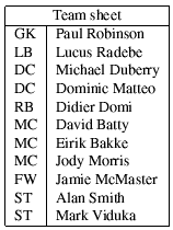
The the command for this looks like this: \multicolumn{num_cols}{alignment}{contents}. num_cols is the number of subsequent columns to merge; alignment is pretty obvious, either l, c, or r. And contents is simply the actual data you want to be contained within that cell. A simple example:

\begin{tabular}{|l|l|} \hline \multicolumn{2}{|c|}{Team sheet} \\ \hline GK & Paul Robinson \\ LB & Lucus Radebe \\ DC & Michael Duberry \\ DC & Dominic Matteo \\ RB & Didier Domi \\ MC & David Batty \\ MC & Eirik Bakke \\ MC & Jody Morris \\ FW & Jamie McMaster \\ ST & Alan Smith \\ ST & Mark Viduka \\ \hline \end{tabular}

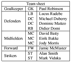
Columns spanning multiple rows

The first thing you need to do is add \usepackage{multirow} to the preamble. This then provides the command needed for spanning rows: \multirow{num_rows}{width}{contents}. The arguments are pretty simple to deduce. With the width parameter, you can specify a fixed with if you wish, or, if you want the natural width (i.e., just wide enough to fit the contents of the column) then simply input an asterisk (*). This approach was used for the following example:

\begin{tabular}{|l|l|l|} \hline \multicolumn{3}{|c|}{Team sheet} \\ \hline Goalkeeper & GK & Paul Robinson \\ \hline \multirow{4}{*}{Defenders} & LB & Lucus Radebe \\ & DC & Michael Duberry \\ & DC & Dominic Matteo \\ & RB & Didier Domi \\ \hline \multirow{3}{*}{Midfielders} & MC & David Batty \\ & MC & Eirik Bakke \\ & MC & Jody Morris \\ \hline Forward & FW & Jamie McMaster \\ \hline \multirow{2}{*}{Strikers} & ST & Alan Smith \\ & ST & Mark Viduka \\ \hline \end{tabular}

The main thing to note when using \multirow is that for the subsequent rows that are to be spanned, a blank entry for the appropriate cells have to be inserted.

Summary

That's about it for basic tables in my opinion. After you experiment, you do quickly get up to scratch. I must admit, the table syntax in Latex can look rather messy, and so seeing new examples can look confusing. But hopefully, enough has been covered here so that you can create any table you are likely to need for your papers. Unsurprisingly, Latex has plenty more up its sleeve, so expect a follow up tutorial covering more advanced features in the near future.

Files: basic.tex | basic.pdf | wrapped.tex | wrapped.pdf | tabular_star.tex | tabular_star.pdf | specifier.tex | specifier.pdf | spanning.tex | spanning.pdf

Last updated: November 5, 2011

« Back to LaTeX tutorials.

LaTeX/Tables

< LaTeX

Jump to: navigation, search

LaTeX

In academic writing, tables are a common feature, often for summarizing results from research. It is therefore a skill that needs mastering in order to produce quality papers.
However, if there is one area about LaTeX that is the least intuitive, then this is it. Basic tables are not too taxing, but you will quickly notice that anything more advanced can take a fair bit of construction. So, we start slowly and build up from there.
Workaround: You might save lots of time by building tables using specialized software and exporting them in LaTeX format. The following plugins and libraries are available for some popular software:

• calc2latex: for OpenOffice.org Calc spreadsheets,
• excel2latex: for Microsoft Office Excel,
• matrix2latex: for MATLAB,
• matrix2latex: for Python and MATLAB,
• latex-tools: a Ruby library,
• xtable: a library for R,
• org-mode: for Emacs users, org-mode tables can be used inline in LaTeX documents, see [1] for a tutorial.
• Emacs Align Commands: while not a workaround per se, the align commands can clean up a messy LaTeX table.

Contents 1 Floating with table 2 The tabular environment 2.1 Basic examples 2.2 Column specification using >{\cmd} and <{\cmd} 2.3 Text wrapping in tables 2.4 Text justification in tables 2.5 Other environments inside tables 2.6 Defining multiple columns 2.7 @-expressions 3 Spanning 3.1 Rows spanning multiple columns 3.2 Columns spanning multiple rows 3.3 Spanning in both directions simultaneously 4 Resize tables 5 Sideways tables 6 Alternate Row Colors in Tables 7 Colors of individual Cells 8 Partial Vertical Lines 9 Space between rows 10 The table environment - captioning etc 11 The tabular* environment - controlling table width 12 The tabularx package - simple column stretching 13 Vertically centered images 14 Professional tables 15 Adding rule spacing above or below \hline and \cline commands 16 Tables with different font size 17 Table with legend 18 Need more complicated features? 19 Summary 20 References

Floating with table

It is highly recommended to place a tabular-environment only in the table-environment, which is able to float and add a label and caption.

\begin{table}[position specifier]
\centering
\begin{tabular}{|l|}
... your table ...
\end{tabular}
\caption{This table shows some data}
\label{tab:myfirsttable}
\end{table}

The captions show now up in the list of tables, if displayed.
You can set the optional parameter position specifier to define the position of the table, where it should be placed. The following characters are all possible placements. Using sequences of it define your "wishlist" to LaTeX.

h	here
t	top
b	bottom
p	page

Default is tbp, which means that it is by default placed on the top of the page. If it's not possible, its placed on the bottom and last possibility is to place it with other floating environments on an extra page. You can force LaTeX to use one given position. E.g. [!h] forces LaTeX to place it exactly where you place it (Except when it's really impossible, e.g you place a table here and this place would be the last line on a page). Centering the table horizontally works using the \centering-command just after opening the table-environment.
More informations about floating environments, captions etc. can be found in Floats, Figures and Captions.

The tabular environment

The tabular environment can be used to typeset tables with optional horizontal and vertical lines. LaTeX determines the width of the columns automatically.
The first line of the environment has the form: \begin{tabular}[pos]{table spec}
The table spec argument tells LaTeX the alignment to be used in each column and the vertical lines to insert.
The number of columns does not need to be specified as it is inferred by looking at the number of arguments provided. It is also possible to add vertical lines between the columns here. The following symbols are available to describe the table columns (some of them require that the package array has been loaded):

l	left-justified column
c	centered column
r	right-justified column
p{width}	paragraph column with text vertically aligned at the top
m{width}	paragraph column with text vertically aligned in the middle (requires array package)
b{width}	paragraph column with text vertically aligned at the bottom (requires array package)
|	vertical line
||	double vertical line

By default, if the text in a column is too wide for the page, LaTeX won’t automatically wrap it. Using p{width} you can define a special type of column which will wrap-around the text as in a normal paragraph. You can pass the width using any unit supported by LaTeX, such as pt and cm, or command lengths, such as \textwidth.You can find a complete list in appendix Useful Measurement Macros.

The optional parameter pos can be used to specify the vertical position of the table relative to the baseline of the surrounding text. In most cases, you will not need this option. It becomes relevant only if your table is not in a paragraph of its own. You can use the following letters:

b	bottom
c	center (default)
t	top

In the first line you have pointed out how many columns you want, their alignment and the vertical lines to separate them. Once in the environment, you have to introduce the text you want, separating between cells and introducing new lines. The commands you have to use are the following:

&	column separator
\\	start new row (additional space may be specified after \\ using square brackets, such as \\[6pt])
\hline	horizontal line
\newline	start a new line within a cell (in a paragraph column)
\cline{i-j}	partial horizontal line beginning in column i and ending in column j

Note, any white space inserted between these commands is purely down to ones' preferences. I personally add spaces between to make it easier to read.

Basic examples

This example shows how to create a simple table in LaTeX. It is a three-by-three table, but without any lines.

\begin{tabular}{ l c r }   1 & 2 & 3 \\   4 & 5 & 6 \\   7 & 8 & 9 \\ \end{tabular}

Expanding upon that by including some vertical lines:

\begin{tabular}{ l | c || r }   1 & 2 & 3 \\   4 & 5 & 6 \\   7 & 8 & 9 \\ \end{tabular}

To add horizontal lines to the very top and bottom edges of the table:

\begin{tabular}{ l | c || r }   \hline                         1 & 2 & 3 \\   4 & 5 & 6 \\   7 & 8 & 9 \\   \hline \end{tabular}

And finally, to add lines between all rows, as well as centering (notice the use of the center environment - of course, the result of this is not obvious from the preview on this web page):

\begin{center}   \begin{tabular}{ l | c || r }     \hline     1 & 2 & 3 \\ \hline     4 & 5 & 6 \\ \hline     7 & 8 & 9 \\     \hline   \end{tabular} \end{center}

\begin{tabular}{|r|l|}   \hline   7C0 & hexadecimal \\   3700 & octal \\ \cline{2-2}   11111000000 & binary \\   \hline \hline   1984 & decimal \\   \hline \end{tabular}

Column specification using >{\cmd} and <{\cmd}

The column specification can be altered using the array package. This is done in the argument of the tabular environment using >{\command} for commands executed right before each column element and <{\command} for commands to be executed right after each column element. As an example: to get a column in math mode enter: \begin{tabular}{>{$}c<{$}}. Another example is changing the font: \begin{tabular}{>{\small}c} to print the column in a small font.
The argument of the > and < specifications must be correctly balanced when it comes to { and } characters. This means that >{\bfseries} is valid, while >{\textbf} will not work and >{\textbf{} is not valid. If there is the need to use the text of the table as an argument (for instance, using the \textbf to produce bold text), one should use the \bgroup and \egroup commands: >{\textbf\bgroup}c<{\egroup} produces the intended effect. This works only for some basic LaTeX commands. For other commands, such as \underline to underline text, it is necessary to temporarily store the column text in a box using lrbox. First, you must define such a box with \newsavebox{\boxname} and then you can define:
>{\begin{lrbox}{\boxname}}%
l%
<{\end{lrbox}%
  \underline{\unhbox\boxname}}%
 }
This stores the text in a box and afterwards, takes the text out of the box with \unhbox (this destroys the box, if the box is needed again one should use \unhcopy instead) and passing it to \underline. (For LaTeX2e, you may want to use \usebox{\boxname} instead of \unhbox\boxname.)
This same trick done with \raisebox instead of \underline can force all lines in a table to have equal height, instead of the natural varying height that can occur when e.g. math terms or superscripts occur in the text.
Here is an example showing the use of both p{...} and >{\centering} :
\begin{tabular}{>{\centering}p{3.5cm}<{\centering}p{3.5cm}}
Geometry  & Algebra
\tabularnewline
\hline
 Points & Addition
\tabularnewline
 Spheres & Multiplication
\end{tabular}
Note the use of \tabularnewline instead of \\ to avoid a Misplaced \noalign error.

Text wrapping in tables

LaTeX's algorithms for formatting tables have a few shortcomings. One is that it will not automatically wrap text in cells, even if it overruns the width of the page. For columns that you know will contain a certain amount of text, then it is recommended that you use the p attribute and specify the desired width of the column (although it may take some trial-and-error to get the result you want). Use the m attribute to have the lines aligned toward the middle of the box and the b attribute to align along the bottom of the box.
Here is a practical example. The following code creates two tables with the same code; the only difference is that the last column of the second one has a defined width of 5 centimeters, while in the first one we didn't specify any width. Compiling this code:
\documentclass{article}

\usepackage[english]{babel}

\begin{document}

Without specifying width for last column:

\begin{center}
    \begin{tabular}{ | l | l | l | l |}
    \hline
    Day & Min Temp & Max Temp & Summary \\ \hline
    Monday & 11C & 22C & A clear day with lots of sunshine.
    However, the strong breeze will bring down the temperatures. \\ \hline
    Tuesday & 9C & 19C & Cloudy with rain, across many northern regions. Clear spells
    across most of Scotland and Northern Ireland,
    but rain reaching the far northwest. \\ \hline
    Wednesday & 10C & 21C & Rain will still linger for the morning.
    Conditions will improve by early afternoon and continue
    throughout the evening. \\
    \hline
    \end{tabular}
\end{center}

With width specified:

\begin{center}
    \begin{tabular}{ | l | l | l | p{5cm} |}
    \hline
    Day & Min Temp & Max Temp & Summary \\ \hline
    Monday & 11C & 22C & A clear day with lots of sunshine.
    However, the strong breeze will bring down the temperatures. \\ \hline
    Tuesday & 9C & 19C & Cloudy with rain, across many northern regions. Clear spells
    across most of Scotland and Northern Ireland,
    but rain reaching the far northwest. \\ \hline
    Wednesday & 10C & 21C & Rain will still linger for the morning.
    Conditions will improve by early afternoon and continue
    throughout the evening. \\
    \hline
    \end{tabular}
\end{center}

\end{document}
You get the following output:

Note that the first table is cropped: The output is wider than the page width.

Text justification in tables

On rare occasions, it might be necessary to stretch every row in a table to the natural width of its longest line, for instance when one has the same text in two languages and wishes to present these next to each other with lines synching up. A tabular environment helps control where lines should break, but cannot justify the text, which leads to ragged right edges. The eqparbox package provides the command \eqmakebox which is like \makebox but instead of a width argument, it takes a tag. During compilation it bookkeeps which \eqmakebox with a certain tag contains the widest text and can stretch all \eqmakeboxes with the same tag to that width. Combined with the array package, one can define a column specifier that justifies the text in all lines: (See the documentation of the eqparbox package for more details.)
\newsavebox{\tstretchbox}
\newcolumntype{S}[1]{%
 >{\begin{lrbox}{\tstretchbox}}%
 l%
 <{\end{lrbox}%
   \eqmakebox[#1][s]{\unhcopy\tstretchbox}}%
  }

Other environments inside tables

If you use some LaTeX environments inside table cells, like verbatim or enumerate
\begin{tabular}{| c | c |}
        \hline
        \begin{verbatim}
        code
        \end{verbatim}
        & description
        \\ \hline
\end{tabular}
you might encounter errors similar to

! LaTeX Error: Something's wrong--perhaps a missing \item.

To solve this problem, change column specifier to "paragraph" (p, m or b).
\begin{tabular}{| m{5cm} | c |}

Defining multiple columns

It is possible to define many identical columns at once using the *{num}{str} syntax.
This is particularly useful when your table has many columns.
Here is a table with six centered columns flanked by a single column on each side:

\begin{tabular}{l*{6}{c}r} Team              & P & W & D & L & F  & A & Pts \\ \hline Manchester United & 6 & 4 & 0 & 2 & 10 & 5 & 12  \\ Celtic            & 6 & 3 & 0 & 3 &  8 & 9 &  9  \\ Benfica           & 6 & 2 & 1 & 3 &  7 & 8 &  7  \\ FC Copenhagen     & 6 & 2 & 1 & 2 &  5 & 8 &  7  \\ \end{tabular}

@-expressions

The column separator can be specified with the @{...} construct.
It typically takes some text as its argument, and when appended to a column, it will automatically insert that text into each cell in that column before the actual data for that cell. This command kills the inter-column space and replaces it with whatever is between the curly braces. To add space, use @{\hspace{width}}.
Admittedly, this is not that clear, and so will require a few examples to clarify. Sometimes, it is desirable in scientific tables to have the numbers aligned on the decimal point. This can be achieved by doing the following:

\begin{tabular}{r@{.}l}   3   & 14159 \\   16  & 2     \\   123 & 456   \\ \end{tabular}

Note that the headers should be enclosed in \multicolumn{2}{l}{HEADER}.
Alternatively, to center the column on the decimal separator the dcolumn package may be used, which provides a new column specifier for floating point data.
The space-suppressing qualities of the @-expression actually make it quite useful for manipulating the horizontal spacing between columns. Given a basic table, and varying the column descriptions:
\begin{tabular}{|l|l|}
  \hline
  stuff & stuff \\ \hline
  stuff & stuff \\
  \hline
\end{tabular}

{|l|l|}
{|@{}l|l@{}|}
{|@{}l@{}|l@{}|}
{|@{}l@{}|@{}l@{}|}

Spanning

To complete this tutorial, we take a quick look at how to generate slightly more complex tables. Unsurprisingly, the commands necessary have to be embedded within the table data itself.

Rows spanning multiple columns

The command for this looks like this: \multicolumn{num_cols}{alignment}{contents}. num_cols is the number of subsequent columns to merge; alignment is either l, c, r, or to have text wrapping specifiy a width p{5.0cm} . And contents is simply the actual data you want to be contained within that cell. A simple example:

\begin{tabular}{|l|l|}   \hline   \multicolumn{2}{|c|}{Team sheet} \\   \hline   GK & Paul Robinson \\   LB & Lucus Radebe \\   DC & Michael Duberry \\   DC & Dominic Matteo \\   RB & Didier Domi \\   MC & David Batty \\   MC & Eirik Bakke \\   MC & Jody Morris \\   FW & Jamie McMaster \\   ST & Alan Smith \\   ST & Mark Viduka \\   \hline \end{tabular}

Columns spanning multiple rows

The first thing you need to do is add \usepackage{multirow} to the preamble^[1]. This then provides the command needed for spanning rows: \multirow{num_rows}{width}{contents}. The arguments are pretty simple to deduce (* for the width means the content's natural width).

... \usepackage{multirow} ... \begin{tabular}{|l|l|l|} \hline \multicolumn{3}{|c|}{Team sheet} \\ \hline Goalkeeper & GK & Paul Robinson \\ \hline \multirow{4}{*}{Defenders} & LB & Lucus Radebe \\  & DC & Michael Duberry \\  & DC & Dominic Matteo \\  & RB & Didier Domi \\ \hline \multirow{3}{*}{Midfielders} & MC & David Batty \\  & MC & Eirik Bakke \\  & MC & Jody Morris \\ \hline Forward & FW & Jamie McMaster \\ \hline \multirow{2}{*}{Strikers} & ST & Alan Smith \\  & ST & Mark Viduka \\ \hline \end{tabular}

The main thing to note when using \multirow is that a blank entry must be inserted for each appropriate cell in each subsequent row to be spanned.
If there is no data for a cell, just don't type anything, but you still need the "&" separating it from the next column's data. The astute reader will already have deduced that for a table of columns, there must always be ampersands in each row. The exception to this is when \multicolumn and \multirow are used to create cells which span multiple columns or rows.

Spanning in both directions simultaneously

Here is a nontrivial example of how to use spanning in both directions simultaneously and have the borders of the cells drawn correctly:

\usepackage{multirow} \begin{tabular}{cc|c|c|c|c|l} \cline{3-6} & & \multicolumn{4}{|c|}{Primes} \\ \cline{3-6} & & 2 & 3 & 5 & 7 \\ \cline{1-6} \multicolumn{1}{|c|}{\multirow{2}{*}{Powers}} & \multicolumn{1}{|c|}{504} & 3 & 2 & 0 & 1 &     \\ \cline{2-6} \multicolumn{1}{|c|}{}                        & \multicolumn{1}{|c|}{540} & 2 & 3 & 1 & 0 &     \\ \cline{1-6} \multicolumn{1}{|c|}{\multirow{2}{*}{Powers}} & \multicolumn{1}{|c|}{gcd} & 2 & 2 & 0 & 0 & min \\ \cline{2-6} \multicolumn{1}{|c|}{}                        & \multicolumn{1}{|c|}{lcm} & 3 & 3 & 1 & 1 & max \\ \cline{1-6} \end{tabular}

The command \multicolumn{1}{|c|}{...} is just used to draw vertical borders both on the left and on the right of the cell. Even when combined with \multirow{2}{*}{...}, it still draws vertical borders that only span the first row. To compensate for that, we add \multicolumn{1}{|c|}{...} in the following rows spanned by the multirow. Note that we cannot just use \hline to draw horizontal lines, since we do not want the line to be drawn over the text that spans several rows. Instead we use the command \cline{2-6} and opt out the first column that contains the text "Powers".
Here is another example exploiting the same ideas to make the familiar and popular "2x2" or double dichotomy:

\begin{tabular}{r|c|c|} \multicolumn{1}{r}{}  &  \multicolumn{1}{c}{noninteractive}  & \multicolumn{1}{c}{interactive} \\ \cline{2-3} massively multiple & Library & University \\ \cline{2-3} one-to-one & Book & Tutor \\ \cline{2-3} \end{tabular}

Resize tables

The command \resizebox{width}{height}{object} can be used with tabular to specify the height and width of a table. The following example shows how to resize a table to 8cm width while maintaining the original width/height ratio.
\resizebox{8cm}{!} {
  \begin{tabular}...
  \end{tabular}}
Alternatively you can use \scalebox{ratio}{object} in the same way but with ratios rather than fixed sizes:
\scalebox{0.7}{
  \begin{tabular}...
  \end{tabular}}
Both \resizebox and \scalebox require the graphicx package.
To tweak the space between columns (LaTeX will by default choose very tight columns), one can alter the column separation: \setlength{\tabcolsep}{5pt}. The default value is 6pt.

Sideways tables

Tables can also be put on their side within a document using the rotating package and the sidewaystable environments in place of the table environment. (NOTE: most DVI viewers do not support displaying rotated text. Convert your document to a PDF to see the result. Most, if not all, PDF viewers do support rotated text.)
\usepackage{rotating}

\begin{sidewaystable}
  \begin{tabular}...
  \end{tabular}
\end{sidewaystable}
When it is desirable to place the rotated table at the exact location where it appears in the source (.tex) file, rotfloat package may be used. Then one can use \begin{sidewaystable}[H] just like for normal tables. The 'H' option can not be used without this package.

Alternate Row Colors in Tables

The xcolor package provides the necessary commands to produce tables with alternate row colors, when loaded with the table option. The command \rowcolors{<starting row>}{<odd color>}{<even color>} has to be specified right before the tabular environment starts.

\documentclass{article} \usepackage[table]{xcolor} \begin{document} \begin{center} \rowcolors{1}{green}{pink} \begin{tabular}{lll} odd     & odd   & odd \\ even    & even  & even\\ odd     & odd   & odd \\ even    & even  & even\\ \end{tabular} \end{center} \end{document}

The command \hiderowcolors is available to deactivate highlighting from a specified row until the end of the table. Highlighting can be reactivated within the table via the \showrowcolors command. If while using these commands you experience "misplaced \noalign errors" then use the commands at the very beginning or end of a row in your tabular (e.g., "\hiderowcolors odd & odd & odd \\" or "odd & odd & odd \\\showrowcolors").

Colors of individual Cells

As above this uses the xcolor package.
% Include this somewhere in your document
\usepackage[table]{xcolor}

% Enter this in the cell you wish to color a light grey.
% NB: the word 'gray' here denotes the grayscale color scheme, not the color grey. '0.9' denotes how dark the grey is.
\cellcolor[gray]{0.9}
% The following will color the cell red.
\cellcolor{red}

Partial Vertical Lines

Adding a partial vertical line to an individual cell:

\begin{tabular}{ l c r }   \hline   1 & 2 & 3 \\ \hline   4 & 5 & \multicolumn{1}{r|}{6}  \\ \hline   7 & 8 & 9 \\ \hline \end{tabular}

Removing part of a vertical line in a particular cell:

\begin{tabular}{ | l | c | r | }   \hline   1 & 2 & 3 \\ \hline   4 & 5 & \multicolumn{1}{r}{6} \\ \hline   7 & 8 & 9 \\ \hline \end{tabular}

Space between rows

Re-define the \arraystretch command to set the space between rows:

\renewcommand{\arraystretch}{1.5}

Default value is 1.0.

The table environment - captioning etc

The tabular environment doesn't cover all that you need to do with tables. For example, you might want a caption for your table. For this and other reasons, you should typically place your tabular environment inside a table environment:
\begin{table}
  \caption{Performance at peak F-measure}
  \begin{tabular}{| r | r || c | c | c |}

      ...

  \end{tabular}
\end{table}
Why do the two different environments exist? Think of it this way: The tabular environment is concerned with arranging elements in a tabular grid, while the table environment represents the table more conceptually. This explains why it isn't tabular but table that provides for captioning (because the caption isn't displayed in the grid-like layout).
A table environment has a lot of similarities with a figure environment, in the way the "floating" is handled etc. For instance you can specify its placement in the page with the option [placement], the valid values are any combination of (order is not important):

h	where the table is declared (here)
t	at the top of the page
b	at the bottom of the page
p	on a dedicated page of floats
!	override the default float restrictions. E.g., the maximum size allowed of a b float is normally quite small; if you want a large one, you need this ! parameter as well.

The default is [tbp]. If you want to place a table in the place where it's declared, do not just write [h]; if the table cannot fit (because the text is near the bottom of the page, say) it will float to a dedicated page of floats (as if it were a p float) which can be some distance away in the document. A good rule of thumb is to always use htbp until the document is finished, at which stage the final float parameters can be fine-tuned.
The table environment is also useful when you want to have a list of tables at the beginning or end of your document with the command \listoftables; it enables making cross-references to the table with:
You may refer to table~\ref{my_table} for an example.

...

\begin{table}
  \begin{tabular}
     ...
  \end{tabular}
  \caption{An example of table}
  \label{my_table}
\end{table}

The tabular* environment - controlling table width

This is basically a slight extension on the original tabular version, although it requires an extra argument (before the column descriptions) to specify the preferred width of the table.

\begin{tabular*}{0.75\textwidth}{ | c | c | c | r | }   \hline   label 1 & label 2 & label 3 & label 4 \\   \hline   item 1  & item 2  & item 3  & item 4  \\   \hline \end{tabular*}

However, that may not look quite as intended. The columns are still at their natural width (just wide enough to fit their contents) while the rows are as wide as the table width specified. If you do not like this default, you must also explicitly insert extra column space. LaTeX has rubber lengths, which, unlike others, are not fixed. LaTeX can dynamically decide how long the lengths should be. So, an example of this is the following.
\begin{tabular*}{0.75\textwidth}{@{\extracolsep{\fill}} | c | c | c | r | }
  \hline
  label 1 & label 2 & label 3 & label 4 \\
  \hline
  item 1  & item 2  & item 3  & item 4  \\
  \hline
\end{tabular*}

You will notice the @{...} construct added at the beginning of the column description. Within it is the \extracolsep command, which requires a width. A fixed width could have been used. However, by using a rubber length, such as \fill, the columns are automatically spaced evenly.

The tabularx package - simple column stretching

This package provides a table environment called tabularx which is similar to the tabular* environment, except that it has a new column specifier X (in uppercase). The column(s) specified with this specifier will be stretched to make the table as wide as specified, greatly simplifying the creation of tables.

\usepackage{tabularx} ... \begin{tabularx}{\textwidth}{ |X|X|X|X| }   \hline   label 1 & label 2 & label 3 & label 4 \\   \hline   item 1  & item 2  & item 3  & item 4  \\   \hline \end{tabularx}

The content provided for the boxes is treated as for a p column, except that the width is calculated automatically. If you use the package array, you may also apply any >{\cmd} or <{\cmd} command to achieve specific behavior (like \centering, or \raggedright\arraybackslash) as described previously.
Another option is the use of \newcolumntype in order to get selected columns formatted in a different way. It defines a new column specifier, e.g. R (in uppercase). In this example, the second and fourth column is adjusted in a different way (\raggedleft):

\usepackage{tabularx} ... \newcolumntype{R}{>{\raggedleft\arraybackslash}X}% \begin{tabularx}{\textwidth}{ |l|R|l|R| }   \hline   label 1 & label 2 & label 3 & label 4 \\   \hline   item 1  & item 2  & item 3  & item 4  \\   \hline \end{tabularx}

Tabularx with rows spanning multiple columns using \multicolumn. The two central columns are posing as one by using the X@{} option. Note that the \multicolumn width (which in this example is 2) should equal the (in this example 1+1) width of the spanned columns:

\usepackage{tabularx} ... \begin{tabularx}{1\textwidth}{|>{\setlength\hsize{1\hsize}\centering}X|>{\setlength\hsize{1\hsize}\raggedleft}X@{} >{\setlength\hsize{1\hsize}\raggedright}X|>{\setlength\hsize{1\hsize}\centering}X|}   \hline Label 1 & \multicolumn{2}{>{\centering\setlength\hsize{2\hsize}}X|}{Label 2} & Label 3\tabularnewline \hline   123  & 123  & 456  & 123  \tabularnewline   \hline   123  & 123  & 456  & 123  \tabularnewline   \hline \end{tabularx}

Vertically centered images

Inserting images into a table row will align it at the top of the cell. By using the array package this problem can be solved. Defining a new columntype will keep the image vertically centered.

\newcolumntype{V}{>{\centering\arraybackslash} m{.4\linewidth} }

Or use a parbox to center the image.

\parbox[c]{1em}{\includegraphics{image.png}}

A raisebox works as well, also allowing to manually fine-tune the alignment with its first parameter.

\raisebox{-.5\height}{\includegraphics{image.png}}

Professional tables

Many professionally typeset books and journals feature simple tables, which have appropriate spacing above and below lines, and almost never use vertical rules. Many examples of LaTeX tables (including this Wikibook) showcase the use of vertical rules (using "|"), and double-rules (using \hline\hline" or "||"), which are regarded as unnecessary and distracting in a professionally published form. The booktabs package is useful for easily providing this professionalism in LaTeX tables, and the documentation also provides guidelines on what constitutes a "good" table.
In brief, the package uses \toprule for the uppermost rule (or line), \midrule for the rules appearing in the middle of the table (such as under the header), and \bottomrule for the lowermost rule. This ensures that the rule weight and spacing are acceptable. In addition, \cmidrule can be used for mid-rules that span specified columns. The following example contrasts the use of booktabs and two equivalent normal LaTeX implementations (the second example requires \usepackage{array} or \usepackage{dcolumn}, and the third example requires \usepackage{booktabs} in the preamble).

Normal LaTeX	Using array	Using booktabs
\begin{tabular}{llr} \hline \multicolumn{2}{c}{Item} \\ \cline{1-2} Animal & Description & Price (\$) \\ \hline Gnat  & per gram & 13.65 \\       & each     &  0.01 \\ Gnu   & stuffed  & 92.50 \\ Emu   & stuffed  & 33.33 \\ Armadillo & frozen & 8.99 \\ \hline \end{tabular}	\usepackage{array} %or \usepackage{dcolumn} ... \begin{tabular}{llr} \firsthline \multicolumn{2}{c}{Item} \\ \cline{1-2} Animal & Description & Price (\$) \\ \hline Gnat  & per gram & 13.65 \\       & each     &  0.01 \\ Gnu   & stuffed  & 92.50 \\ Emu   & stuffed  & 33.33 \\ Armadillo & frozen & 8.99 \\ \lasthline \end{tabular}	\usepackage{booktabs} ... \begin{tabular}{llr} \toprule \multicolumn{2}{c}{Item} \\ \cmidrule(r){1-2} Animal & Description & Price (\$) \\ \midrule Gnat  & per gram & 13.65 \\       & each     &  0.01 \\ Gnu   & stuffed  & 92.50 \\ Emu   & stuffed  & 33.33 \\ Armadillo & frozen & 8.99 \\ \bottomrule \end{tabular}

Usually the need arises for footnotes under a table (and not at the bottom of the page), with a caption properly spaced above the table. These are addressed by the ctable package. It provides the option of a short caption given to be inserted in the list of tables, instead of the actual caption (which may be quite long and inappropriate for the list of tables). The ctable package uses the booktabs package.

Adding rule spacing above or below \hline and \cline commands

An alternative way to adjust the rule spacing is to add \noalign{\smallskip} before or after the \hline and \cline{i-j} commands:
Normal LaTeX
\begin{tabular}{llr}
\hline\noalign{\smallskip}
\multicolumn{2}{c}{Item} \\
\cline{1-2}\noalign{\smallskip}
Animal & Description & Price (\$) \\
\noalign{\smallskip}\hline\noalign{\smallskip}
Gnat  & per gram & 13.65 \\
      & each     &  0.01 \\
Gnu   & stuffed  & 92.50 \\
Emu   & stuffed  & 33.33 \\
Armadillo & frozen & 8.99 \\
\noalign{\smallskip}\hline
\end{tabular}
You may also specify the skip after a line explicitly using glue after the line terminator
\begin{tabular}{|l|l|}
\hline
Mineral & Color \\[1cm]
Ruby & red \\
Sapphire & blue \\
\hline
\end{tabular}

Tables with different font size

A table can be globally switched to a different font size by simply adding the desired size command (here: \footnotesize) after the \begin{table}... statement:
\begin{table}[h]\footnotesize
  \caption{Performance at peak F-measure}
  \begin{tabular}{| r | r || c | c | c |}

      ...

  \end{tabular}
\end{table}
The table caption font size is not affected.
To control the caption font size, see Caption Styles.

Table with legend

To add a legend to a table the caption package can be used. With the caption package a \caption*{...} statement can be added besides the normal \caption{...}.
Example
\begin{table}
  \begin{tabular}{| r | r || c | c | c |}

      ...

  \end{tabular}
  \caption{A normal caption}
  \caption*{
    A legend, even a table can be used
    \begin{tabular}{l l}
      item 1 & explanation 1 \\
    \end{tabular}
  }
\end{table}
The normal caption is needed for labels and references.

Need more complicated features?

Have a look at one of the following packages:

• hhline: do whatever you want with horizontal lines
• array: gives you more freedom on how to define columns
• colortbl: make your table more colorful
• supertabular: for tables that need to stretch over several pages
• longtable: similar to supertab.
  • Note: footnotes do not work properly in a normal tabular environment. If you replace it with a longtable environment, footnotes work properly
• threeparttable makes it possible to put footnotes both within the table and its caption
• xtab: Yet another package for tables that need to span many pages
• tabulary: modified tabular* allowing width of columns set for equal heights
• arydshln: creates dashed horizontal and vertical lines
• ctable: allows for footnotes under table and properly spaced caption above (incorporates booktabs package)
• slashbox: create 2D tables with the first cell containing a description for both axes
• dcolumn: decimal point alignment of numeric cells
• rccol: advanced decimal point alignment of numeric cells with rounding
• numprint: print numbers, in the current mode (text or math) in order to use the correct font, with separators, exponent and/or rounded to a given number of digits. tabular(*), array, tabularx, and longtable environments is supported using all features of numprint
• spreadtab: spread sheets allowing the use of formulae
• siunitx: alignment of tabular entries

Summary

This concludes discussion of basic tables. The table syntax in LaTeX can look rather messy, and new examples can look confusing. But hopefully, enough has been covered here so that a user can create any table needed for their papers. Unsurprisingly, LaTeX has plenty more up its sleeve, so expect a follow-up tutorial covering more advanced features in the near future.

References

1. ↑ Package multirow on CTAN

Previous: List Structures

Index

Next: Formatting

Category:

• LaTeX

What do you think of this page?

Please take a moment to rate this page below. Your feedback is valuable and helps us improve our website.
Reliability:  Completeness:  Neutrality:  Presentation: 

• Log in
• Create account

• Book
• Discussion

• Read
• Edit
• View history

• Main Page
• Help
• Browse
• Cookbook
• Wikijunior
• Featured books
• Recent changes
• Donations
• Random book

Community

• Reading room
• Community portal
• Bulletin Board
• Help out!
• Policies and guidelines
• Contact us

Toolbox

In other languages

• Français
• Nederlands
• Polski

Sister projects

Print/export

• This page was last modified on 8 June 2012, at 14:23.
• Text is available under the Creative Commons Attribution-ShareAlike License; additional terms may apply. See Terms of Use for details.

• Privacy policy
• About Wikibooks
• Disclaimers
• Mobile view

• 
•