Sunday, March 31, 2013

randon transform and Real time tracking


http://www.ece.neu.edu/groups/rcl/projects/back_projection/phantom.jpg


Image Projections and the Radon Transform

DSP BORDER
Image Projections and the Radon Transform


The basic problem of tomography is given a set of 1-D projections and the angles at which these projections were taken, how do we recontruct the 2-D image from which these projections were taken? The first thing we did was to look at the nature of the projecitons. Fig(1) - 
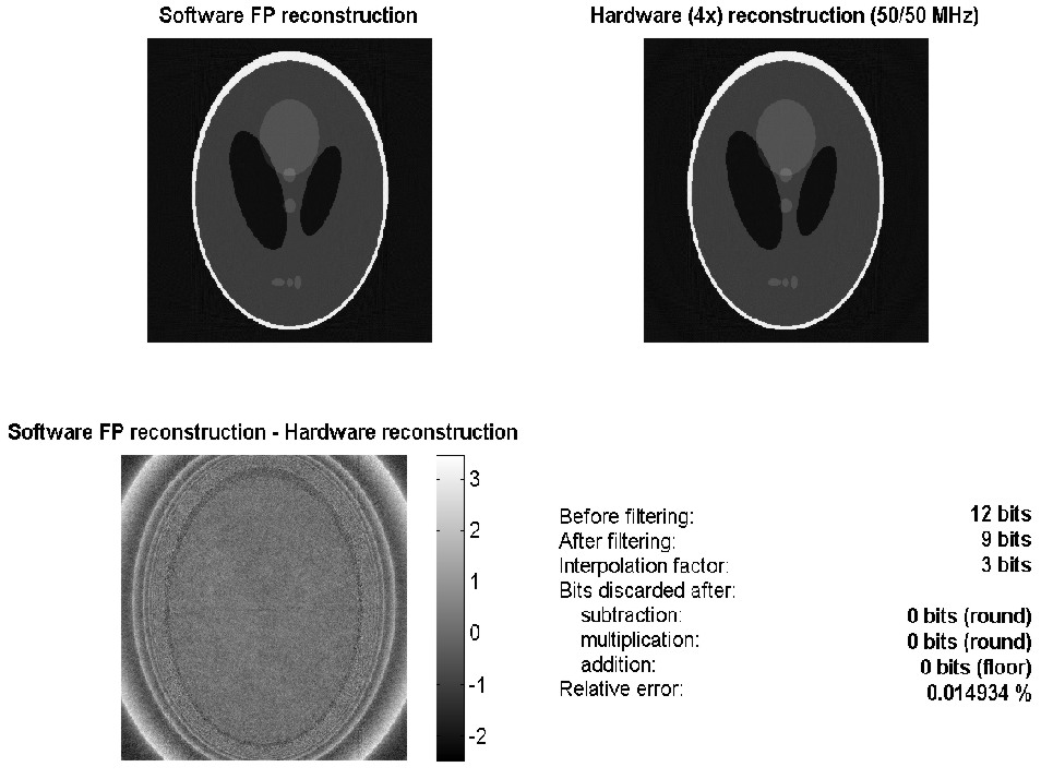
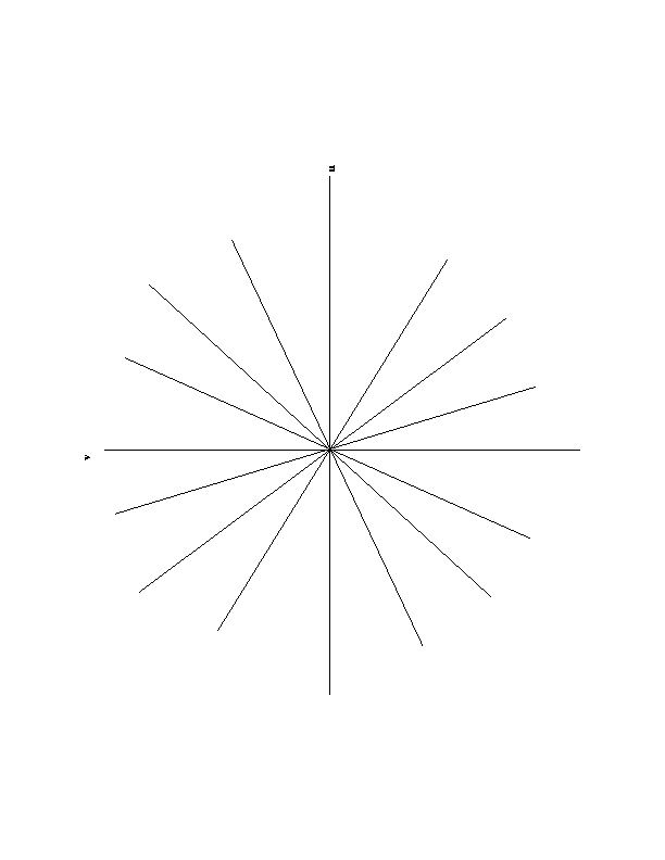
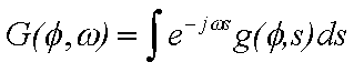
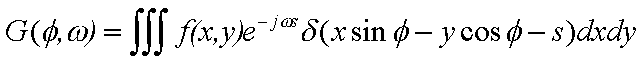
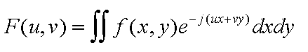
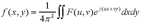
Define g(phi,s) as a 1-D projection at an angle . g(phi,s) is the line integral of the image intensity, f(x,y), along a line l that is distance s from the origin and at angle phi off the x-axis.
Eqn(1)
All points on this line satisfy the equation : x*sin(phi) - y*cos(phi) = s Therefore, the projection function g(phi,s) can be rewritten as
Eqn(2)
The collection of these g(phi,s) at all phi is called the Radon Transform of image f(x,y). To be able to study different reconstruction techniques, we first needed to write a (MATLAB) program that took projections of a known image. Having the original image along with the projections gives us some idea of how well our algorithm performs. The projection code is pretty simple. Basically, we take the image (which is just a matrix of intensities in MATLAB), rotate it, and sum up the intensities. In MATLAB this is easily accomplished with the 'imrotate' and 'sum' commands. First, we zero pad the image so we don't lose anything when we rotate (the images are rectangular so the distance across the diagonal is longer than the distance on a side). Then we rotate the image 90-phi degrees (so that the projection is lined up in the columns) using the 'imrotate' command, and finally summed up the columns using the 'sum' command. The performance of this program was marginal. We did not bother optimizing the code for MATLAB because our main focus was reconstructing the images, not taking projections of them. Filtered Backprojection and the Fourier Slice Theorem
In order to reconstruct the images, we used what is known as the Fourier Slice Theorem. The Slice Theorem tells us that the 1D Fourier Transform of the projection function g(phi,s) is equal to the 2D Fourier Transform of the image evaluated on the line that the projection was taken on (the line that g(phi,0) was calculated from). So now that we know what the 2D Fourier Transform of the image looks like (or at least what it looks like on certain lines and then interpolate), we can simply take the 2D inverse Fourier Transform and have our original image. Fig. 2 - 
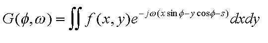
We can show the Fourier Slice Theorem in the following way: The 1D Fourier Transform of g is given by :
Eqn(3)
Now, we subsitute our expression for g(phi,s) (Eqn. 2) into the expression above to get
Eqn(4)
We can use the sifting property of the Dirac delta function to simplify to
Eqn(5)
Now, if we recall the definition of the 2D Fourier Transform of f
Eqn(6)
we can see that that Eqn 5. is just F(u,v) evaluated at u = w*sin(phi) and v = -w*cos(phi), which is the line that the projection g(phi,s) was taken on! Now that we have shown the Fourier Slice Theorem, we can continue with the math to gain further insight. First, recall the definition for the 2D inverse Fourier Transform
Eqn(7)
Now, we make a change of variable from rectangular to polar coordinates and replace F(phi,w) with G(phi,w) we get
Eqn(8)
where |w| is the determinant of the Jacobian of the change of variable from rectangular to polar coordinates. We now have a relationship between the projection functions and the image we are trying to recontruct, so we can easily write a program to do the reconstruction. Notice that we have to multiply our projections by |w| in the Fourier domain. This product
Eqn(9)
is called the filtered back projection at angle phi. If we look at Fig. 2, we can see that we have a lot of information at low frequencies (near the origin), and not as much at high frequencies. The |w|, which is a ramp filter, compensates for this. Below, we show our phantom object reconstructed from 1, 4, 8, 15, and 60 filtered back projections. With only one back projection, not much information about the original image is revealed. 
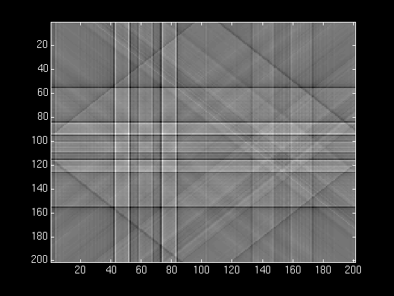
With 4 back projections, we can see some of the basic features start to emerge. The two squares on the left side start to come in, and the main ellise looks like a diamond. 
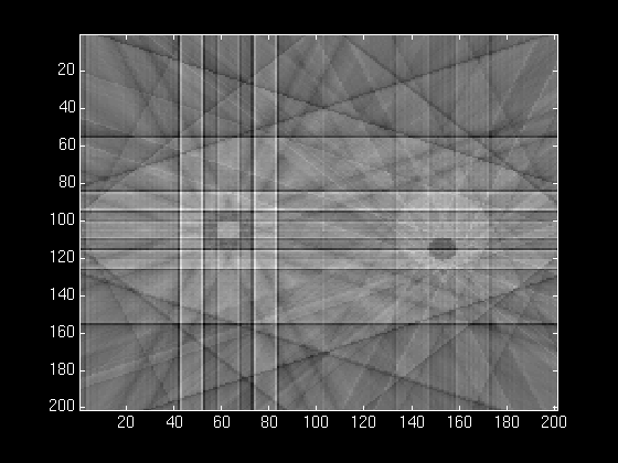
At 8 back projections, our image is finally starting to take shape. We can see the squares and the circles well, and we can make out the basic shape of the main ellipse. 
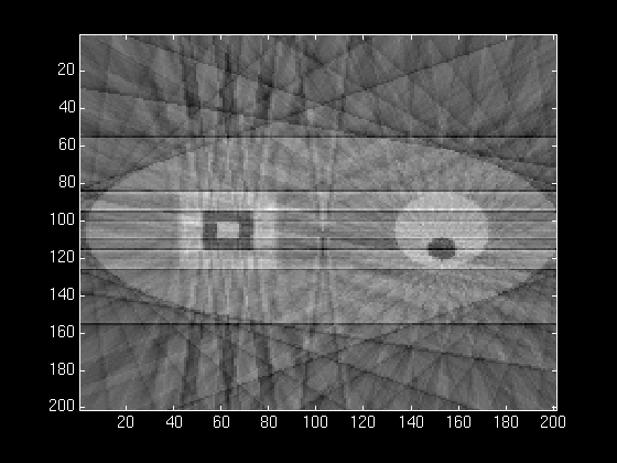
With 15 back projections, we can see the bounds of the main ellipse very well, and the squares and cirlces are well defined. The lines in the center of the ellipse appear as blurry triangles. Also, we have a lot of undesired residuals in the back ground (outside the main ellipse). 
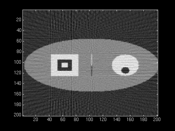
At 60 back projections, our reconstructed image looks very nice. We still have some patterns outside the ellipse, and there are streaks from the edge of the squares all the way out to the edge of the image. These appear because the edge of the square is such a sharp transistion at 0 and 90 degrees, that when we pass the projections through the ramp filter, there are sharp spikes in the filtered projections. These never quite seem to get smoothed out. The MATLAB code for the filtered back projections worked very nicely. The basic algorithm we used for filtered back projections was : 
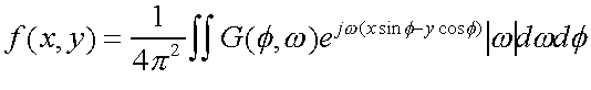
f(x,y) is the image we are trying to recontruct, q(phi,s) is the filtered back projection at angle phi. Initialize f(x,y) For each p do For each (x,y) do Find the contributing spot in the filtered back projection that corresponds to (x,y) at angle phi, in other words s = xsin(phi) - ycos(phi) f(x,y) = f(x,y) + q(phi,s); end end Since we used MATLAB to do all the image processing, we were able to vectorize the computations, and cut out the entire inner loop (which is really 2 loops, one for x and one for y). The run times were blazingly fast, our algorithm took about .2 seconds per back projection on our phantom when running on a SPARC 5.
DSP BORDER
On to the next page... Back to the front page.


Ref:
http://www.slideshare.net/VanyaVabrina/radon-transform-image-analysis
http://www.ece.neu.edu/groups/rcl/projects/back_projection/phantom.jpg
http://hesperia.gsfc.nasa.gov/rhessidatacenter/imaging/back_projection.html
 http://www.clear.rice.edu/elec431/projects96/DSP/bpanalysis.html


real time object tracking and Interlace and progressive
http://www.slideshare.net/VanyaVabrina/


IMAGE procesing sclide


http://www.scribd.com/resmi_ng/documents

back projection  

Web definitions
Histogram equalization is a method in image processing of contrast adjustment using the image's histogram..

http://www.scribd.com/doc/86629205/Image-Reconstruction-from-Projections
http://www.scribd.com/doc/86594495/11/Fundamental-Coding-Theorems
http://www.scribd.com/doc/86594495/Image-Compression-Fundamentals
http://www.scribd.com/doc/86595009/Image-Compression-Coding-Schemes
http://www.scribd.com/doc/86595009/1/Error-Free-Compression
http://www.scribd.com/doc/86595009/2/Variable-Length-Coding
http://www.scribd.com/doc/86595009/3/Lempel-Ziv-Welch-LZW-Coding

http://www.scribd.com/doc/86595009/4/Bit-Plane-Coding
http://www.scribd.com/doc/86595009/5/Constant-Area-Coding
http://www.scribd.com/doc/86595009/6/Lossless-Predictive-Coding
http://www.scribd.com/doc/86595009/7/Lossy-Predictive-Coding
http://www.scribd.com/doc/86595009/8/Transform-Coding
http://www.scribd.com/doc/86595009/9/Wavelet-Coding
 http://www.scribd.com/doc/86595009/10/JPEG
http://www.scribd.com/doc/86595009/11/JPEG-2000

http://www.scribd.com/doc/86595009/12/For-Self-Study

 http://www.scribd.com/doc/86594495/4/Interpixel-Redundancy
http://www.scribd.com/doc/86240949/Digital-Image-Processing-Fundamentals
http://www.scribd.com/doc/86248966/Image-Enhancement-Frequency-Domain


http://www.scribd.com/doc/86252580/Image-Restoration
www.scribd.com/doc/86252580/3/Periodic-Noise
www.scribd.com/doc/86252580/9/Notch-Filters
www.scribd.com/doc/86252580/10/Optimum-Notch-Filtering


www.scribd.com/doc/86252580/11/Convolution
http://www.scribd.com/doc/86252580/5/Bandreject-Filters
http://www.scribd.com/doc/86252580/6/Butterworth-Bandreject-filters
http://www.scribd.com/doc/86252580/17/Wiener-MMSE-Filtering
www.scribd.com/doc/86252580/16/Inverse-Filtering


http://www.scribd.com/doc/86241949/3/Brightness-Discrimination
http://www.scribd.com/doc/86245257/Linear-Systems


http://inst.eecs.berkeley.edu/~ee225b/fa12/lectures/lec1-Introduction.pdf
http://inst.eecs.berkeley.edu/~ee225b/fa12/lectures/
http://home.engineering.iastate.edu/~namrata/EE528_Spring07/Class_Schedule.html
http://www.cs.tut.fi/~karen/dip2_96.html


https://www.cosic.esat.kuleuven.be/vandermeulen/slides/van-der-meulen-seminar_2011-12-07.pdf

ICA AND PCA book


http://www.amazon.com/Introduction-Spectral-Analysis-Petre-Stoica/dp/0132584190

Introduction to Spectral Analysis [Paperback]

Petre Stoica , Randolph L. Moses

Friday, March 29, 2013

Color Models and Color Spaces

 what is  Demosaicing?
A demosaicing (also de-mosaicing or demosaicking) algorithm is a digital image process used to reconstruct a full color image from the incomplete color samples output from an image sensor overlaid with a color filter array (CFA). It is also known as CFA interpolation or color reconstruction.

 what is color filter arrary?
 bayer color and bayer filter

Color Space and Color Profiles

This page presents an in-depth discussion of the methods used to reproduce color in digital photography.
What's a color model?
What's a color space?
What's a color profile?

http://dpbestflow.org/color/color-space-and-color-profiles#model
http://www.lightillusion.com/forums/index.php?action=vthread&forum=8&topic=50
http://www.cs.rit.edu/~ncs/color/a_spaces.html
http://en.wikipedia.org/wiki/Color_space
http://www.mathworks.in/help/images/converting-color-data-between-color-spaces.html

http://www.siliconimaging.com/RGB%20Bayer.htm

http://www.edn.com/design/integrated-circuit-design/4312122/Converter-translates-Bayer-raw-data-to-RGB-format
http://stackoverflow.com/questions/7598854/how-do-i-convert-bayer-to-rgb-using-opencv-and-vice-versa
 http://stackoverflow.com/questions/10403841/convert-12-bit-bayer-image-to-8-bit-rgb-using-opencv
 http://en.wikipedia.org/wiki/Bayer_filter
http://en.wikipedia.org/wiki/Bayes_filter
 http://en.wikipedia.org/wiki/Demosaicing
 http://www.helicontech.co.il/?id=bayer-rgb

gamut : complete range or scope of something.
subtle: so delicate, sharp.


REf :

https://developer.apple.com/library/mac/#documentation/Cocoa/Conceptual/DrawColor/Concepts/AboutColorSpaces.html

http://en.wikipedia.org/wiki/Color_filter_array

About Color Spaces

A color space describes an abstract, multidimensional environment in which any particular color can be defined. The following sections summarize the basic concepts and terminology of color spaces and discusses how Cocoa implements them.
Some of the information presented here is adapted from Color Management Overview. For a thorough description of color and color spaces, see that document.


Color Models and Color Spaces

The human eye apprehends color as light in a fairly narrow band of the electromagnetic spectrum. The biology of the eye makes it particularly receptive to red, blue, and green light. Humans can visualize a broad range of colors through mixtures of these three primary colors.
A color model is a geometric or mathematical framework that attempts to describe the colors we see. It uses numerical values pinned to dimensions of the model to represent the visible spectrum of color. A color model gives us a method for describing, classifying, comparing, and ordering colors.
A color space is a practical adaptation of a color model that specifies a gamut of colors that can be produced using that model. The color model determines the relationship between values, and the color space defines the absolute meaning of those values as colors. These values, called components, are in most instances floating-point values between 0.0 and 1.0.

Gray, RGB, and CYMK Color Spaces

The simplest color space is the gray space (sometimes also called the white space). The gray space has a single dimension or component, ranging from pure white to pure black; it is used for grayscale printing.
RGB is a three-dimensional color model whose name (as with most color spaces and color models) represents its components—in this case red, green, and blue. RGB-based color spaces are additive, meaning that the three primary colors red, green, and blue are added together in various proportions of intensity to create the colors of the visible spectrum. RGB color spaces are used for devices such as color displays and scanners.
On the other hand, color spaces based on the CYM color model are subtractive. The letters in the model name stand for the components cyan, yellow, and magenta. The major color space based on CYM is CYMK; the “K” in its name stands for the key color, which is black. The subtractive color theory, which underlies CYM, holds that various levels of cyan, magenta, and yellow absorb or “subtract” a portion of the spectrum of the white light illuminating an object. The color of an object is the result of the lights that are not absorbed by the object. The black in the CYMK color space is used to compensate for the interaction of the three primary colors on white paper. The CYMK color space is most commonly used for color printers and similar output devices.
As Figure 1 illustrates, the RGB and CYM color models are complementary, with one being additive and the other subtractive (the red corner in this model representation is hidden from view).
Figure 1  The RGB and CYM color models
The RGB and CYM color models
Two important and related transformations of the RGB color model are the HSV and HLS color spaces. Instead of making red, green, and blue the operative components of the space, these spaces describe colors in terms more natural to an artist:
  • HSV—hue, saturation, value (also known as HSB, where “B” represents brightness)
  • HLS—hue, lightness, saturation
The HSV/B and HLS spaces use models that assign values to these components in conical geometries, as illustrated in Figure 2.
Figure 2  The HSV and HLB color models
The HSV and HLB color models
The hue component in both spaces is a measurement in degrees of color in a spectrum formed into a circle. The values are incremented in a counterclockwise direction: a hue value of zero specifies red, a hue value of 120 indicates green, and so on. In both the HSB and HLS spaces, the saturation component measures color intensity (making the major difference, for example, between tan and brown). The lightness and value (or brightness) components of the different spaces are almost identical. They measure the absence of light—or black—that is part of particular color.
The color panel used in Mac apps has a color-wheel pane that simulates the HSB model (Figure 3).
Figure 3  The color-wheel pane of the color panel
The color-wheel pane of the color panel

Device-Independent Color Spaces

Color spaces based on RGB and CYM color models can be device-dependent or device-independent. Colors from device-dependent color spaces are dependent on the physical characteristics of devices such as monitors (RGB and grayscale) and printers (CYMK) as well as the properties of materials such as ink and paper. Even the age of a device can affect the color it produces. Device-dependent color spaces are limited by the gamut, or range, of colors that a particular device is capable of. Consequently, colors in a device-dependent color space can appear different when rendered by different devices of the same general type.
One can also note subtle color differences among color spaces in the same color-model “family.” For example, the RGB color model has many RGB color spaces, such as ColorMatch, Adobe RGB, sRGB, and ProPhoto RGB. You can assign the same RGB component values to profiles that describe these different RGB color spaces. The color from each color space looks different when rendered, but the numeric values and model are the same.
Some color spaces can express color in a way that is independent of any device. The colors of these device-independent color space are more accurate representations of the colors perceived by the human eye. They derive from the response of the retina to the three primary stimuli of visible light. Many device-independent color spaces result from work carried out by the Commission Internationale d’Eclairage (CIE) and for that reason are also called CIE-based color spaces. Three of the more important CIE-based spaces are XYZ, Yxy, and L*a*b*. Figure 4 depicts the L*a*b* color space.
Figure 4  The L*a*b* color space
The L*a*b* color space
One important use for device-independent color spaces is to convert a color in one device-dependent color space to a reasonably approximate color in a different device-dependent color space. For example, if a program wanted to ensure that a photo displayed on a color monitor (using a RGB color space) was accurately rendered on a printer (using a CYMK color space), it might use a device-independent color space as an interchange space.

Wednesday, March 27, 2013

why shouldn't i eat non veg

No one should living by killing.
Because it takes small persons to beats a defense less animals
 because no animals deserve to die for yours testebubs


because they defense less.
 when animal feel pain they  screams too
no matter how u slices still it is flash.

heart diseases in child hood.


http://www.youtube.com/watch?v=eP1mRpQ28Kw
http://www.messagefrommasters.com/veg/osho-on-nonvegetarian-food-ashram.html
http://www.spiritualresearchfoundation.org/articles/id/spiritualresearch/spiritualscience/veg-or-non-veg#3Effectsofdietonman
http://forum.spiritualindia.org/veg-or-nonveg-to-eat-or-not-to-eat-t31645.0.html
http://www.createdebate.com/debate/show/Vegetarianism_vs_Non_vegetarianism_3

point

 Change in you life 
1. You don't have right to talk about any body ! if he or she doesn't allow  to you to use speak (degree of f   freedom. )
2. Stop talk nonsense think  and -ve thing about others.
3. Don't try to connect by link each other ,in starting it feels good but in a longer rang it irritates and break relationship.
4.never excite any time , in the next moment you feel bore and sad  .

Have to follow these point Points
Zero ego.
Zero angry.
Zero exception. ( never wait or thought to get any thing from others)
Hundred percent confidence .
Enjoy each moment with 100 percent efficiency ( means in this moment this is the best i can do  not possible more than this)
Be happy and make happy others.
Don't be arrogant and stubborn
Never blame and give pain to others.
Praise others and never comment  others
 Be honest , truth fullness and simple.
Believe your self and
Respect  others, other language, other religion, others culture, other country.

Orthogonal Frequency Division Multiplexing


http://www.wirelesscommunication.nl/reference/chaptr05/ofdm/ofdm.htm

Orthogonal Frequency Division Multiplexing

Orthogonal Frequency Division Multiplexing (OFDM) is special form of multi-carrier modulation, patented in 1970. It is particularly suited for transmission over a dispersive channel. (See further discussion of MCM over wireless channel.)In a multipath channel, most conventional modulation techniques are sensitive to intersymbol interference unless the channel symbol rate is small compared to the delay spread of the channel. OFDM is significantly less sensitive to intersymbol interference, because a special set of signals is used to build the composite transmitted signal. The basic idea is that each bit occupies a frequency-time window which ensures little or no distortion of the waveform. In practice, it means that bits are transmitted in parallel over a number of frequency-nonselective channels. Applications of OFDM are found in
  • Digital Audio Broadcasting (DAB) and
  • Digital Video Broadcasting over the terrestrial network: Digital Terrestrial Television Broadcasting (DTTB). In the DTTB OFDM transmission standard, about 2,000 to 8,000 subcarriers are used.
  • UMTS. The UMTS Forum is selecting an appropriate radio solution for the third generation mobile standard, as a successor to GSM. OFDM is one of the five competing proposals.
  • Wireless LANs. OFDM is used in HIPERLAN Phase II, which supports 20 Mbit/s in propagation environments with delay spreads up to 1 msecond.

Figure: Signal spectrum of an OFDM signal, which consists of the spectra of many bits, in parallel. Rectangular pulses in time domain produce sinc-functions in frequency domain.
  • Above: signal spectrum as transmitted.
  • Below: as received in over a dispersive, time-invariant channel.
The effect of multipath scattering on OFDM differs from what happens to other forms of modulation. A qualitative description and mathematical description of OFDM is presented by Dusan Matic. Jean-Paul Linnartz reviews the effects of a Doppler spread and the associated rapid channel variations. Dusan Matic also studied the system design aspects of OFDM at mm-wavelengths.

 Exercise

Consider two subcarrier signals, modulated with rectangular pulse shape of duration T. For which frequency offsets are the signals orthogonal? What is the effect of a mild channel dispersion on the orthogonality of the signals? Are the signals still orthogonal if the channel is changing rapidly?

Coded OFDM

Multi-Carrier Modulation on its own is not the solution to the problems of communication over unreliable multipath channels. The channel time dispersion will excessively attenuate some subcarriers such that the throughput on these sub-channels would be unacceptable small. Only if the joint signal of many subcarriers is processed appropriately, the diversity advantages of MCM can be exploited. The need for coding across subcarriers was addressed by Sari et al. warning against overly enthusiastic pursuit of MCM. The advantages of frequency-domain implementations of equalizers (using an FFT) should not be mistaken for an "inherent" diversity gain of OFDM, which may not exist.
Coding for wireless
Turbo coding for OFDM
Frequency Diversity
 

In an OFDM transmitter, blocks of k incoming bits are encoded into n channel bits. Before transmission, an n-point Inverse-FFT operation is performed. When the signals at the I-FFT output are transmitted sequentially, each of the n channel bits appears at a different (subcarrier) frequency. Such coding across subcarriers is necessary. If one subcarrier experiences deep fading, this leads to erasure of the bit on this subcarrier.
But of course coding across subcarriers is not the only mechanism that can be invoked to combat dispersion or to exploit diversity. Other possibilities are
  • Interleaving in frequency or time domain with coding in the other domain,
  • The use of different signal constellations at different frequencies, i.e., adapting the subcarrier bit rate to the channel state,
  • Signal spreading over various subcarriers, e.g., according to a linear matrix operation, as is proposed in Orthogonal Multi-Carrier Code Division Multiplexing.
If in a point-to-point MCM link, the receiver and the transmitter can cooperate by adaptively distributing of their power budget over the individual subcarriers. For instance, the signal-to-noise ratios selected according to Gallager's water-pouring theorem can (under certain conditions) be proved to be optimum. Efficient loading of the various subcarriers can for instance significantly enhance the performance of MCM over twisted pair telephone subscriber loops with crosstalk from other nearby copper pairs.

Implementational Aspects

Figure: OFDM transmitter using an (inverse) Fast Fourier Transform (FFT).


  • OFDM is not a constant-envelope modulation method. Therefore transmit power amplifiers must be highly linear.
  • OFDM receiver performance is very sensitive to phase noise.
  • Synchronization to an OFDM signal also requires frame synchronization, to support an FFT operation at the receiver.


Single Frequency Networks

OFDM allows very efficient frequency reuse. Transmitters broadcasting the same program can use the same frequency in a Single Frequency Network.

Code Division Multiple Access

OFDM can be combined with CDMA transmission, e.g. in Multi-Carrier CDMA.

Channel Modeling

Many channel simulation models follow the narrowband model. Wideband channels are often simulated by extending the model assuming multiple time-delayed resolvable paths. This allows the simulation of the channel impulse response, including its stochastic behavior. To determine the performance of an multicarrier, OFDM or MC-CDMA system, another approach can be to model a set of fading subchannels. Considering a single subcarrier, the channel may be modelled as a narrowband fading channel, for instance with Rician or Rayleigh amplitude distributions. The collection of multiple subcarriers can be modelled as a set of mutually dependentfading channels. In such model, it is important to address correlation of the fading of various subchannels using the models of delay spread and coherence bandwidth. See a discussion of such model. Also: read about thediscrete-frequency model for OFDM with Delay spread and Doppler.
 Listen to an MP3 audio program about on OFDM, featuring Jeff Anderson (SONY), Geert Awater (Lucent), Helmut Boelsckei (Stanford U.) and Jean-Paul Linnartz (Philips).

 SMIL
Synchronous
Multimedia
Animated audio tutorial on OFDM and MC-CDMA

http://blog.oureducation.in/important-questions-on-ofdm/


1)  What is OFDM?
Ans: 
OFDM  (Orthogonal Frequency Division Multiplexing) is a broadband multicarrier modulation method that offers superior performance and benefits over older, more traditional single-carrier modulation methods because it is a better fit with today’s high-speed data requirements and operation in the UHF and microwave spectrum.
2) How does OFDM work?
Ans: 
OFDM is based on the concept of frequency-division multiplexing (FDD), the method of transmitting multiple data streams over a common broadband medium. That medium could be radio spectrum, coax cable, twisted pair, or fiber-optic cable. Each data stream is modulated onto multiple adjacent carriers within the bandwidth of the medium, and all are transmitted simultaneously. A good example of such a system is cable TV, which transmits many parallel channels of video and audio over a single fiber-optic cable and coax cable.
3) Why has there been all the interest in OFDM in the past few years?
Ans: 
OFDM has been adopted as the modulation method of choice for practically all the new wireless technologies being used and developed today. It is perhaps the most spectrally efficient method discovered so far, and it mitigates the severe problem of multipath propagation that causes massive data errors and loss of signal in the microwave and UHF spectrum.
4) Name some of the wireless technologiesthat use OFDM?
Ans: 
The list is long and impressive. First, it is used for digital radio broadcasting. It is used in TV broadcasting.You will also find it in wireless local-area networks (LANs) like Wi-Fi. The wideband wireless metro-area network (MAN) technology WiMAX uses OFDM. And, the almost completed 4G cellular technology standard Long-Term Evolution (LTE) uses OFDM. The high-speed short-range technology known as Ultra-Wideband (UWB) uses an OFDM standard set by the WiMedia Alliance. OFDM is also used in wired communications like power-line networking technology. One of the first successful and most widespread uses of OFDM was in data modems connected to telephone lines. ADSL and VDSL used for Internet access use a form of OFDM known as discrete multi-tone (DMT). And, there are other less well known examples in the military and satellite worlds.
5) How is OFDM implemented in the real world?
Ans: 
OFDM is accomplished with digital signal processing (DSP). We can program the IFFT and FFT math functions on any fast PC, but it is usually done with a DSP IC or an appropriately programmed FPGA or some hardwired digital logic. With today’s super-fast chips, even complex math routines like FFT are relatively easy to implement. In brief, we can put it all on a single chip.
6) What are the benefits of using OFDM?
Ans: 
The first reason is spectral efficiency, also called bandwidth efficiency. What that term really means is that you can transmit more data faster in a given bandwidth in the presence of noise. The measure of spectral efficiency is bits per second per Hertz, or bps/Hz. For a given chunk of spectrum space, different modulation methods will give you widely varying maximum data rates for a given bit error rate (BER) and noise level. Simple digital modulation methods like amplitude shift keying (ASK) and frequency shift keying (FSK) are only fair but simple. BPSK and QPSK are much better. QAM is very good but more subject to noise and low signal levels. Code division multiple access (CDMA) methods are even better. But none is better than OFDM when it comes to getting the maximum data capacity out of a given channel. It comes close to the so called Shannon limit that defines channel capacity C in bits per second (bps) as
C = B * log2(1 + S/N)Here, B is the bandwidth of the channel in hertz, and S/N is the power signal-to-noise ratio. With spectrum scarce or just plain expensive, spectral efficiency has become the holy grail in wireless.
7) What else makes OFDM so good?
Ans: 
OFDM is highly resistant to the multipath problem in high-frequency wireless. Very short-wavelength signals normally travel in a straight line (line of sight, or LOS) from the transmit antenna to the receive antenna. Yet trees, buildings, cars, planes, hills, water towers, and even people will reflect some of the radiated signal. These reflections are copies of the original signal that also go to the receive antenna. If the time delays of the reflections are in the same range as the bit or symbol periods of the data signal, then the reflected signals will add to the direct signal and create cancellations or other anomalies. The result is what we usually call Raleigh fading.
8) What are the downsides to OFDM?
Ans: 
Like anything else, OFDM is not perfect. It is very complex, making it more expensive to implement. However, modern semiconductor technology makes it pretty easy. OFDM is also sensitive to carrier frequency variations. To overcome this problem, OFDM systems transmit pilot carriers along with the subcarriers for synchronization at the receiver. Another disadvantage is that an OFDM signal has a high peak to average power ratio. As a result, the complex OFDM signal requires linear amplification. That means greater inefficiency in the RF power amplifiers and more power consumption.
9) What is OFMDA?
Ans: 
The A stands for access. It means that OFDM is not only a great modulation method, it also can provide multiple access to a common bandwidth or channel to multiple users. You are probably familiar with multiple access methods like frequency-division multiplexing (FDM) and time division multiplexing (TDM). CDMA, the widely used cellular technology, digitally codes each digital signal to be transmitted and then transmits them all in the same spectrum. Because of their random nature, they just appear as low-level noise to one another. The digital coding lets the receiver sort the individual signal out later. OFDMA permits multiple users to share a common bandwidth with essentially the same benefits.
10) Is there anything better than OFDM?
Ans: 
Not right now. What makes OFDM even better is MIMO, the multiple-input multiple-output antenna technology.

http://www.glassdoor.com/Interview/Qualcomm-Modem-Systems-Test-Engineer-Interview-Questions-EI_IE640.0,8_KO9,36.htm

CDMA basics operation, OFDM basic principle, Importance of orthogonaility in OFDM, How is Orthogonality achieved, Cyclic prefix in OFDM,
MIMO basics, Antenna Diversity concept.
Interview Details – I applied for the position in mid August and got the invitation for the phone interview after a month. The phone interview lasted around 45 minutes. It was purely technical, covering all aspects of MIMO and OFDM. Make sure you know what you are taking about because they cover the concepts well in depth and throwing out buzz words might land you in trouble.
The interviewer was very nice and explained about the position after the technical round.
He offered me to come on site straightway. One important tip is to make sure you ask good questions about the position at the end.

On site interview process is very exhaustive and in depth. I had 8 rounds, one HR and 7 technical. All the interviewers were very nice, professional and supportive. The interview process covered all the basics of wireless communications including fading, modulation techniques, interleaving, source coding/channel coding, MIMO equalizers, fundamentals of TCP/IP, digital communications, signal processing and C programming (particularly pointers and linked lists)
In between the interviews, they take you out for lunch. Make you you strike an intelligent conversation during that time and ask relevant questions.
Also make sure you are very thorough with your resume as they can ask about any experience mentioned their.
Interview Question – Take a random sequence of bits and perform source coding using Huffman code.
Write an optimization function for a 4 way traffic intersection, where vehicles are coming in from all directions. [Hint: Think cars as client in need of service arriving at an arrival rate and traffic light as the server process with a service rate]
Drive the bit error rate of BPSK.
Write a regular expression in Perl to search for a string pattern.( this was unexpected since I had told them I did not know perl )
How would you test a Modem if you get complaints from field about cell phones not working. Describe the test cases.
   Answer Question

Interview Details – Had technical phone interview with qualcomm's staffing manager. It was an resume based interview. Interviewer asked me about my project, got a real-time situation question from the project, that what would happen if given some conditions. I had a question about jamming and anti-jamming. Then one question from probability and unions. And one question in selective frequency fading.
Interview Details – It was a day long interview. Started with an HR round followed by six technical rounds. They interviewers were really kind and encouraging. Since I come from a Wireless Communications background, most of the questions were related to communications and networks.
Interview Question – Few questions are :
- Basic communication block diagram and then going in-depth about each block
- Types of fading and methods to combat
- Modulation techniques
- CDMA concepts like handover, power control - why is it used ?
- OFDM concepts, how is cyclic prefix done ?
- TCP / IP
- Some basic socket programming
- Puzzles (Not math ones) Just on the spot thinking kinda puzzles
- Rake receivers
- Why Rayleigh fading ? ?
   
Interview Details – Asked about 4G LTE technology, MIMO, basics of DSP z-transform, AWGN channel, OFDM. If you are perfect in these areas it is easy to ace the interview. Be perfect with LTE technology.


http://blog.oureducation.in/modulation-and-demodulation-based-interview-questions/

Q1. What is modulation and demodulation ?
Ans1. Modulation is the process of altering the characteristics of the amplitude, frequency, or phase angle of the high-frequency signal in accordance with the instantaneous value of the modulating wave.
Modulation
Demodulation is the process of extracting the original information signal from a modulated carrier signal.
Demodulation
Q2. Explain the need of modulation and demodulation ?
Ans2. Modulation is required to send the information over long distances as low frequency signals are not able to cover large area.
While demodulation is required to get back the information sent at the receiving side.
Q3. What is analog modulation and state various techniques?
Ans3. In it, the modulating technique is applied to the analog information signal. Its various techniques are:
• Amplitude modulation(AM)
• Frequency modulation(FM)
• Phase modulation(PM)
Q4. Why frequency modulation is better then amplitude modulation?
Ans4. Modulation is better as it provide more resistance to noise as compared to demodulation.
Q5. What is digital modulation and state various techniques?
Ans5. We can consider it as conversion of analog to digital signal. Its various techniques are:
• PSK- Phase shift keying
• ASK- Amplitude shift keying
• FSK- Frequency shift keying
• QAM- Quadrature amplitude modulation
Q6. State the techniques of demodulation?
Ans6. There are several ways of demodulation depending on how parameters of the carrier signal, such as amplitude, frequency or phase.
• For a signal modulated with a linear modulation, like AM, we can use a synchronous detector.
• For a signal modulated with an angular modulation, we must use an FM demodulator or a PM demodulator.
Q7. Which type of modulation is used in TV transmission?
Ans7. Vegestial side band modulation (VSBM).
Q8. What is the difference between detector and demodulator?
Ans8. A detector is a device that recovers information of interest contained in a modulated wave.
Demodulation is updated form of detector which extracts the original information from a modulated carrier wave.
Q9. What is depth of modulation?
Ans9. It refers to the ratio of the unmodulated carrier amplitude to the amplitude deviation for which the modulated carrier wave reaches its minimum value.
Q10. What is the difference between coherent and non-coherent demodulation?
Ans10. In case of coherent, carrier used for demodulation purpose is in phase and frequency synchronism with carrier used for modulation purpose while for non-coherent, it is not in synchronism.

http://ebookbrowse.com/el/elec3100-2012


http://www.scribd.com/doc/61839369/Digital-Communications-VIVA

There are essentially two aspects to Coding theory:
  1. Data compression (or, source coding)
  2. Error correction (or, channel coding).

Coding theory is the study of the properties of codes and their fitness for a specific application. Codes are used for data compressioncryptographyerror-correction and more recently also fornetwork coding. Codes are studied by various scientific disciplines—such as information theoryelectrical engineeringmathematics, and computer science—for the purpose of designing efficient and reliable data transmission methods. This typically involves the removal of redundancy and the correction (or detection) of errors in the transmitted data.

 A typical music CD uses the Reed-Solomoncode to correct for scratches and dust. In this application the transmission channel is the CD itself. 
Data modems, telephone transmissions, and NASA all employ channel coding techniques to get the bits through, for example the turbo code and LDPC codes
Algebraic coding theory is basically divided into two major types of codes:[citation needed]
  1. Linear block codes
  2. Convolutional codes.


There are many types of linear block codes, such as
  1. Cyclic codes (e.g., Hamming codes)
  2. Repetition codes
  3. Parity codes
  4. Polynomial codes (e.g., BCH codes)
  5. Reed–Solomon codes
  6. Algebraic geometric codes
  7. Reed–Muller codes
  8. Perfect codes.


Differentiat between source coding and channel coding?


Source Coding : this is done to reduce the size of the information (data compression) being transmitted and conserve the available bandwidth. This process reduces redundancy. 
e.g. zipping files, video coding (H.264, AVS-China, Dirac) etc.
e.g. huff man codes, rle codes, arithmetic coding etc.


Channel Coding : this is done to reduce errors during transmission of data along the channel from the source to the destination. This process adds to the redundancy of data.

e.g. Turbo codes, convolutional codes, block coding etc.


Channel coding - This coding is usually done to reduce the errors during thetransmission of information in the channel. Usually, these codes add redundancy to the information.

Source coding - This coding is done at the terminals to reduce the bandwidth used for communication. Usually, 
these codes reduce the redundancy.

Sunday, March 24, 2013

synthetic telepathy


http://phys.org/news137863959.html#jCp

http://www.ocf.berkeley.edu/~anandk/neuro/poster.pdf

http://www.mindcontrol.se/?page_id=1509

http://beamsandstruts.com/bits-a-pieces/item/1026-telepathy

http://www.sheldrake.org/Articles%26Papers/papers/telepathy/pdf/experiment_tests.pdf


http://www.sheldrake.org/Research/telepathy/

Scientists to study synthetic telepathy

The research could lead to a communication system that would benefit soldiers on the battlefield and paralysis and stroke patients, according to lead researcher Michael D’Zmura, chair of the UCI Department of Cognitive Sciences. “Thanks to this generous grant we can work with experts in automatic speech recognition and in brain imaging at other universities to research a brain-computer interface with applications in military, medical and commercial settings,” D’Zmura says. The brain-computer interface would use a noninvasive brain imaging technology like electroencephalography to let people communicate thoughts to each other. For example, a soldier would “think” a message to be transmitted and a computer-based speech recognition system would decode the EEG signals. The decoded thoughts, in essence translated brain waves, are transmitted using a system that points in the direction of the intended target. “Such a system would require extensive training for anyone using it to send and receive messages,” D’Zmura says. “Initially, communication would be based on a limited set of words or phrases that are recognized by the system; it would involve more complex language and speech as the technology is developed further.” D’Zmura will collaborate with UCI cognitive science professors Ramesh Srinivasan, Gregory Hickok and Kourosh Saberi. Joining the team are researchers Richard Stern and Vijayakumar Bhagavatula from Carnegie Mellon’s Department of Electrical and Computer Engineering and David Poeppel from the University of Maryland’s Department of Linguistics. The grant comes from the U.S. Department of Defense’s Multidisciplinary University Research Initiative program, which supports research involving more than one science and engineering discipline. Its goal is to develop applications for military and commercial uses.

Read more at: http://phys.org/news137863959.html#jCp

synthetic telepathy

automatic speech recognition and in brain imaging at other universities to research a brain-computer interface with applications in military, medical and commercial settings,” D’Zmura says.

Read more at: http://phys.org/news137863959.html#jCp


Topics in Research 
Brain-computer interface
Imagined speech
cognitive science


Related
EEG


Research collage

 UCI cognitive science professors Ramesh Srinivasan, Gregory Hickok and Kourosh Saberi

Richard Stern and Vijayakumar Bhagavatula  from Carnegie Mellon’s Department of Electrical and Computer Engineering 
and David Poeppel from the University of Maryland’s Department of Linguistics.

Lead researcher Michael D’Zmura, chair of the UCI Department of Cognitive Sciences.

Read more at: http://phys.org/news137863959.html#jCp


Neural science course
http://www.ece.cmu.edu/courses/items/18698.html

he brain is among the most complex systems ever studied. Underlying the brain's ability to process sensory information and drive motor actions is a network of roughly 1011 neurons, each making 103 connections with other neurons. Modern statistical and machine learning tools are needed to interpret the plethora of neural data being collected, both for (1) furthering our understanding of how the brain works, and (2) designing biomedical devices that interface with the brain. This course will cover a range of statistical methods and their application to neural data analysis. The statistical topics include latent variable models, dynamical systems, point processes, dimensionality reduction, Bayesian inference, and spectral analysis. The neuroscience applications include neural decoding, firing rate estimation, neural system characterization, sensorimotor control, spike sorting, and field potential analysis.


Special Topics in Applies Physics: Neural Technology, Sensing, and Stimulation

Neural Technology, Sensing, and Stimulation
This course gives engineering insight into the operation of excitable cells, as well as circuitry for sensing and stimulation nerves. Initial background topics include diffusion, osmosis, drift, and mediated transport, culminating in the Nernst equation of cell potential. We will then explore models of the nerve, including electrical circuit models and the Hodgkin-Huxley mathematical model. Finally, we will explore aspects of inducing a nerve to fire artificially, and cover circuit topologies for sensing action potentials and for stimulating nerves. If time allows, we will discuss other aspects of medical device design. Students will complete a neural stimulator or sensor design project.
Prerequisites: 18-220 or equivalent, or an understanding of basic circuits, differential equations, and electricity and magnetism. Some review of circuit theory will be provided for those who need it.


New Topics in Signal Processing: Network Science: Modeling and Inference

Do you ever wonder how seeming successfully ants forage for rich sources of food, bees move a beehive to more suitable locations, flocks of birds fly in formation? How come a tree falling in Ohio causes fifty five million people in the Northeast of the US and Canada to loose their electrical power? Why the actions of a few in an once in the financial district in London impact so significantly the World financial markets? Why do critical infrastructures, e.g., cellular and mobile networks, fail in times of crisis, when they are most needed? How do bot-nets spread and compromise millions of computers in the internet? Can companies understand the viral behavior of their three million (did you say eighty million) (mobile) customers? These and others are background and motivational examples that guide us in this course whose goal is the study of relatively dumb agents that sense, process, and cooperate locally but whose collective, coordinated activity leads to the emergence of complex behaviors. Among others, the course will develop basic tools to understand: i) the modeling of these highly networked, large scale structures (e.g., colonies of agents, networks of physical systems, cyber physical systems ii) how to predict the behavior of these networked systems iii) how to derive and study the properties (e.g., convergence and performance) of distributed algorithms for inference and data assimilation. The course will develop graph representations and introduce tools from spectral graph theory, will cover the basics from queueing theory, Markov point processes, and stochastic networks to predict behaviors under several types of stress conditions and asymptotic regimens, and will explore consensus algorithms and several classes of distributed inference algorithms operating under infrastructure failures (intermittent random sensor and channel failures,) different resource constraints (e.g., power or bandwidth,) or random protocols (e.g., gossip.) The course is essentially self-contained. There will be a mix of homework, midterm exams, and projects. Students will take an active role by exploring examples of applications and applying network science concepts to fully develop the analysis of their preferred applications.
Pre-requisites: Probability theory.


http://www.uni-oldenburg.de/en/academic-research/main-areas-of-research/neurosensors/

 molecular biology or image processing. With their interdisciplinary approach they investigate the processes through which the brain produces an internal image of the world on the basis of the stimuli it receives from the sensory organs, whereby the focus is on the interaction between different sensations.


 Advanced Digital Signal Processing

This course will examine a number of advanced topics and applications in one-dimensional digital signal processing, with emphasis on optimal signal processing techniques. Topics will include modern spectral estimation, linear prediction, short-time Fourier analysis, adaptive filtering, plus selected topics in array processing and homomorphic signal processing, with applications in speech and music processing.
4 hrs. lec.
Prerequisites: 18-491 and 36-217

 Image, Video, and Multimedia

The course is designed to explore video computing algorithms including: image and video compression, steganography, object detection and tracking, motion analysis, 3D display, augmented reality, telepresence, sound recognition, video analytics and video search. The course emphasizes experimenting with the real-world videos. The assignments consist of four projects, readings and presentations

The course studies image processing, image understanding, and video sequence analysis. Image processing deals with deterministic and stochastic image digitization, enhancement. restoration, and reconstruction. This includes image representation, image sampling, image quantization, image transforms (e.g., DFT, DCT, Karhunen-Loeve), stochastic image models (Gauss fields, Markov random fields, AR, ARMA) and histogram modeling. Image understanding covers image multiresolution, edge detection, shape analysis, texture analysis, and recognition. This includes pyramids, wavelets, 2D shape description through contour primitives, and deformable templates (e.g., 'snakes'). Video processing concentrates on motion analysis. This includes the motion estimation methods, e.g., optical flow and block-based methods, and motion segmentation. The course emphasizes experimenting with the application of algorithms to real images and video. Students are encouraged to apply the algorithms presented to problems in a variety of application areas, e.g., synthetic aperture radar images, medical images, entertainment video image, and video compression.
Section P is for Portugal students only.


Special Topics in Signal Processing: Cognitive Video


Rapidly growing mobile and online videos have enriched our digital lives. They also create great challenges to our computing and networking technologies, ranging from video indexing, analysis, retrieval, to synthesis. The course covers the state-of-the-art of video processing, video understanding, and video interaction technologies, including video annotation, eye tracking, motion capture, telepresence, event and object detection, augmented reality, video summarization, and video interface design. Students will have hands-on experience with devices such as Kinect 3D sensor, Android smartphone, eye tracker, mocap, and infrared camera. The class assignments include labs and a class project.
Pre-requisites: 18290 or instuctor approval, MATLAB or C, Calculus, and matrix computation.


Multimedia Communications: Coding, Systems, and Networking

This course introduces technologies for multimedia communications. We will address how to efficiently represent multimedia data, including video, image, and audio, and how to deliver them over a variety of networks. In the coding aspect, state-of-the-art compression technologies will be presented. Emphasis will be given to a number of standards, including H.26x, MPEG, and JPEG. In the networking aspect, special considerations for sending multimedia over ATM, wireless, and IP networks, such as error resilience and quality of service, will be discussed. The H.32x series, standards for audiovisual communication systems in various network environments, will be described. Current research results in multimedia communications will be reviewed through student seminars in the last weeks of the course.


 Special Topics in Signal Processing: Registration in Bioimaging

This course will cover the fundamentals of image matching (registration) methods with applications to biomedical engineering. As the fundamental step in image data fusion, registration methods have found wide ranging applications in biomedical engineering, as well as other engineering areas, and have become a major topic in image processing research. Specific topics to be covered include manual and automatic landmark-based, intensity-based, rigid, and nonrigid registration methods. Applications to be covered include multi-modal image data fusion, artifact (motion and distortion) correction and estimation, atlas-based segmentation, and computational anatomy. Course work will include Matlab programming exercises, reading of scientific papers, and independent projects. Upon successful completion, the student will be able to develop his/ her own solution to an image processing problem that involves registration.
Prerequisites: 18-396 or permission of the instructor, working knowledge of Matlab, and some image processing experience.
This course is cross listed with 42-708 Special Topics: Registration in Bioimaging


Special Topics in Signal Processing: Design Impletmentation of Speech Recognition Systems


Voice recognition systems invoke concepts from a variety of fields including speech production, algebra, probability and statistics, information theory, linguistics, and various aspects of computer science. Voice recognition has therefore largely been viewed as an advanced science, typically meant for students and researchers who possess the requisite background and motivation.
In this course we take an alternative approach. We present voice recognition systems through the perspective of a novice. Beginning from the very simple problem of matching two strings, we present the algorithms and techniques as a series of intuitive and logical increments, until we arrive at a fully functional continuous speech recognition system.
Following the philosophy that the best way to understand a topic is to work on it, the course will be project oriented, combining formal lectures with required hands-on work. Students will be required to work on a series of projects of increasing complexity. Each project will build on the previous project, such that the incremental complexity of projects will be minimal and eminently doable. At the end of the course, merely by completing the series of projects students would have built their own fully-functional speech recognition systems.
Grading will be based on project completion and presentation.
Prerequisites: Mandatory: Linear Algebra. Basic Probability Theory. Recommended: Signal Processing. Coding Skills: This course will require significant programming form the students. Students must be able to program fluently in at least one language (C, C++, Java, Python, LISP, Matlab are all acceptable).


ML

Signal Processing is the science that deals with extraction of information from signals of various kinds. This has two distinct aspects -- characterization and categorization. Traditionally, signal characterization has been performed with mathematically-driven transforms, while categorization and classification are achieved using statistical tools.
Machine learning aims to design algorithms that learn about the state of the world directly from data.
A increasingly popular trend has been to develop and apply machine learning techniques to both aspects of signal processing, often blurring the distinction between the two.
This course discusses the use of machine learning techniques to process signals. We cover a variety of topics, from data driven approaches for characterization of signals such as audio including speech, images and video, and machine learning methods for a variety of speech and image processing problems.
Prerequisites: Linear Algebra, Basic Probability Theory, Signal Processing and Machine Learning.