or
in the preamble of the document.
Mathematics environments
LaTeX needs to know beforehand that the subsequent text does in fact
contain mathematical elements. This is because LaTeX typesets maths
notation differently than normal text. Therefore, special environments
have been declared for this purpose. They can be distinguished into two
categories depending on how they are presented:
- text - text formulas are displayed in-line, that is, within the body of text where it is declared. e.g., I can say that a + a = 2a within this sentence.
- displayed - displayed formulas are separate from the main text.
As maths require special environments, there are naturally the
appropriate environment names you can use in the standard way. Unlike
most other environments, however, there are some handy shorthands to
declaring your formulas. The following table summarizes them:
| Type |
Environment |
LaTeX shorthand |
TeX shorthand |
| Text |
\begin{math}...\end{math} |
\(...\) |
$...$ |
| Displayed |
\begin{displaymath}...\end{displaymath} or
\begin{equation*}...\end{equation*}[3] |
\[...\] |
$$...$$ |
In order for some operators, such as
\lim or
\sum to be displayed correctly inside some math environments (read
$......$), it might be convenient to write the
\displaystyle
class inside the environment. Doing so might cause the line to be
taller, but will cause exponents and indices to be displayed correctly
for some math operators. For example, the $\sum$ will print a smaller Σ
and $\displaystyle \sum$ will print a bigger one

, like in equation (This only works with AMSMATH package).
Symbols
Mathematics has lots and lots of symbols! If there is one aspect of
maths that is difficult in LaTeX it is trying to remember how to produce
them. There are of course a set of symbols that can be accessed
directly from the keyboard:
+ - = ! / ( ) [ ] < > | ' :
Beyond those listed above, distinct commands must be issued in order to display the desired symbols. And there are
a lot! of Greek letters, set and relations symbols, arrows, binary operators, etc. For example:
\[
\forall x \in X, \quad \exists y \leq \epsilon
\] |
 |
Fortunately, there's a tool that can greatly simplify the search for
the command for a specific symbol. Look for "Detexify" in the
external links section below. Another option would be to look in the "The Comprehensive LaTeX Symbol List" in the
external links section below.
Greek letters
Greek letters are commonly used in mathematics, and they are very easy to type in
math mode.
You just have to type the name of the letter after a backslash: if the
first letter is lowercase, you will get a lowercase Greek letter, if the
first letter is uppercase (and only the first letter), then you will
get an uppercase letter. Note that some uppercase Greek letters look
like Latin ones, so they are not provided by LaTeX (e.g. uppercase
Alpha and
Beta
are just "A" and "B" respectively). Lowercase epsilon, theta, phi, pi,
rho, and sigma are provided in two different versions. The alternate, or
variant, version is created by adding "var" before the name of the letter:
\[
\alpha, \Alpha, \beta, \Beta, \gamma, \Gamma,
\pi, \Pi, \phi, \varphi, \Phi
\] |
α,Α,β,Β,γ,Γ,π,Π,ϕ,φ,Φ |
Scroll down to
#List_of_Mathematical_Symbols for a complete list of Greek symbols.
Operators
An operator is a function that is written as a word: e.g.
trigonometric functions (sin, cos, tan), logarithms and exponentials
(log, exp). LaTeX has many of these defined as commands:
\[
\cos (2\theta) = \cos^2 \theta - \sin^2 \theta
\] |
 |
For certain operators such a
s limits, the subscript is placed underneath the operator:
\[
\lim_{x \to \infty} \exp(-x) = 0
\] |
 |
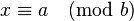
For the
modular operator there are two commands:
\bmod and
\pmod:
\[
a \bmod b
\] |
 |
\[
x \equiv a \pmod b
\] |
 |
Powers and indices
Powers and indices are equivalent to superscripts and subscripts in normal text mode. The caret (
^) character is used to raise something, and the underscore (
_) is for lowering. If more than one expression is raised or lowered, they should be grouped using curly braces (
{ and
}).
\[
k_{n+1} = n^2 + k_n^2 - k_{n-1}
\] |
 |
An underscore (
_) can be used with a vertical bar (
| ) to denote evaluation using subscript notation in mathematics:
\[
f(n) = n^5 + 4n^2 + 2 |_{n=17}
\] |
 |
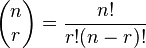
Fractions and Binomials
A fraction is created using the
\frac{numerator}{denominator} command. (for those who need their memories refreshed, that's the
top and
bottom respectively!)
\[
\frac{n!}{k!(n-k)!} = \binom{n}{k}
\] |
 |
It is also possible to use the
\choose command without the
amsmath package:
\[
\frac{n!}{k!(n-k)!} = {n \choose k}
\] |
 |
You can embed fractions within fractions:
\[
\frac{\frac{1}{x}+\frac{1}{y}}{y-z}
\] |
 |
Note that when appearing inside another fraction, or in inline text

, a fraction is noticeably smaller than in displayed mathematics. The
\tfrac and
\dfrac commands
[3] force the use of the respective styles,
\textstyle and
\displaystyle. Similarly, the
\tbinom and
\dbinom commands typeset the binomial coefficient.
Another way to write fractions is to use the
\over command without the
amsmath package:
\[
{n! \over k!(n-k)!} = {n \choose k}
\] |
 |
For relatively simple fractions, it may be more aesthetically pleasing to use
powers and indices:
\[
^3/_7
\] |
 |
If you use them throughout the document, usage of
xfrac package is recommended. This package provides
\sfrac command to create slanted fractions. Usage:
Take \sfrac{1}{2} cup of sugar, \dots
\[
3\times\sfrac{1}{2}=1\sfrac{1}{2}
\]
Take ${}^1/_2$ cup of sugar, \dots
\[
3\times{}^1/_2=1{}^1/_2
\] |
 |
Alternatively, the
nicefrac package provides the
\nicefrac command, whose usage is similar to
\sfrac.
Continued fractions
Continued fractions should be written using
\cfrac command
[3]:
\begin{equation}
x = a_0 + \cfrac{1}{a_1
+ \cfrac{1}{a_2
+ \cfrac{1}{a_3 + a_4}}}\end{equation} |
 |
Multiplication of two numbers
To make multiplication visually similar to a fraction, you can use
nested array. Multiplication of numbers written one behalf other.
\begin{equation}
\frac{
\begin{array}[b]{r}
\left( x_1 x_2 \right)\\
\times \left( x'_1 x'_2 \right)
\end{array}
}{
\left( y_1y_2y_3y_4 \right)
}\end{equation} |
![\frac{
\begin{array}[b]{r}
\left( x_1 x_2 \right)\\
\times \left( x'_1 x'_2 \right)
\end{array}
}{
\left( y_1y_2y_3y_4 \right)
}](http://upload.wikimedia.org/wikibooks/en/math/0/1/e/01e8112dcec7fa9471c1cfaaa4e7cddd.png) |
Roots
The
\sqrt command creates a square root surrounding an expression. It accepts an optional argument specified in square brackets (
[ and
]) to change magnitude:
\[
\sqrt{\frac{a}{b}}
\] |
 |
\[
\sqrt[n]{1+x+x^2+x^3+\ldots}
\] |
![\sqrt[n]{1+x+x^2+x^3+\ldots}](http://upload.wikimedia.org/wikibooks/en/math/9/a/c/9ac55c571b112fba4b527b8b1eb19e17.png) |
Some people prefer writing the square root "closing" it over its
content. This method arguably makes it more clear just what is in the
scope of the root sign. This habit is not normally used while writing
with the computer, but if you still want to change the output of the
square root, LaTeX gives you this possibility. Just add the following
code in the preamble of your document:
% New definition of square root:
% it renames \sqrt as \oldsqrt
\let\oldsqrt\sqrt
% it defines the new \sqrt in terms of the old one
\def\sqrt{\mathpalette\DHLhksqrt}
\def\DHLhksqrt#1#2{%
\setbox0=\hbox{$#1\oldsqrt{#2\,}$}\dimen0=\ht0
\advance\dimen0-0.2\ht0
\setbox2=\hbox{\vrule height\ht0 depth -\dimen0}%
{\box0\lower0.4pt\box2}} |

The new style is on left, the old one on right
|
This TeX code first renames the
\sqrt command as
\oldsqrt, then redefines
\sqrt
in terms of the old one, adding something more. The new square root can
be seen in the picture on the right, compared to the old one.
Unfortunately this code won't work if you want to use multiple roots: if
you try to write
![\sqrt[b]{a}](http://upload.wikimedia.org/wikibooks/en/math/e/0/0/e001d537da149e5ceb715383a72b0f02.png)
as
\sqrt[b]{a}
after you used the code above, you'll just get a wrong output. In other
words, you can redefine the square root this way only if you are not
going to use multiple roots in the whole document.
Sums and integrals
The
\sum and
\int commands insert the sum and integral symbols respectively, with limits specified using the caret (
^) and underscore (
_). The typical notation for sums is:
\[
\sum_{i=1}^{10} t_i
\] |
 |
The limits for the integrals follow the same notation. It's also
important to represent the integration variables with an upright d,
which in math mode is obtained through the \mathrm{} command, and with a
small space separating it from the integrand, which is attained with
the \, command.
\[
\int_0^\infty e^{-x}\,\mathrm{d}x
\] |
 |
There are many other "big" commands which operate in a similar manner:
\sum |
 |
|
\prod |
 |
|
\coprod |
 |
\bigoplus |
 |
|
\bigotimes |
 |
|
\bigodot |
 |
\bigcup |
 |
|
\bigcap |
 |
|
\biguplus |
 |
\bigsqcup |
 |
|
\bigvee |
 |
|
\bigwedge |
 |
\int |
 |
|
\oint |
 |
|
\iint[3] |
 |
\iiint[3] |
 |
|
\iiiint[3] |
 |
|
\idotsint[3] |
 |
For more integral symbols, including those not included by default in the Computer Modern font, try the
esint package.
The
\substack command
[3] allows the use of
\\ to write the limits over multiple lines:
\[
\sum_{\substack{
0<i<m \\
0<j<n
}}
P(i,j)
\] |
 |
If you want the limits of an integral to be specified above and below the symbol (like the sum), use the
\limits command:
\[
\int\limits_a^b
\] |
 |
However if you want this to apply to ALL integrals, it is preferable to specify the
intlimits option when loading the
amsmath package:
| \usepackage[intlimits]{amsmath} |
Subscripts and superscripts in other contexts as well as other parameters to
amsmath package related to them are described in
Advanced Mathematics chapter.
For bigger integrals, you may use personal declarations, or the
bigints package
[4].
Brackets, braces and delimiters
How to use braces in multi line equations is described in the Advanced Mathematics chapter.
The use of delimiters such as brackets soon becomes important when
dealing with anything but the most trivial equations. Without them,
formulas can become ambiguous. Also, special types of mathematical
structures, such as matrices, typically rely on delimiters to enclose
them.
There are a variety of delimiters available for use in LaTeX:
\[
() \, [] \, \{\} \, || \, \|\| \,
\langle\rangle \, \lfloor\rfloor \, \lceil\rceil
\] |
![() \, [] \, \{\} \, || \, \|\| \, \langle\rangle \, \lfloor\rfloor \, \lceil\rceil
\,](http://upload.wikimedia.org/wikibooks/en/math/d/7/a/d7a2a4ce921a29b9c7b255047d3394f1.png) |
Automatic sizing
Very often mathematical features will differ in size, in which case
the delimiters surrounding the expression should vary accordingly. This
can be done automatically using the
\left and
\right commands. Any of the previous delimiters may be used in combination with these:
\[
\left(\frac{x^2}{y^3}\right)
\] |
 |
Curly braces are defined differently by using
\left\{ and
\right\},
\[
\left\{\frac{x^2}{y^3}\right\}
\] |
 |
If a delimiter on only one side of an expression is required, then an
invisible delimiter on the other side may be denoted using a period (
.).
\[
\left.\frac{x^3}{3}\right|_0^1
\] |
 |
Manual sizing
In certain cases, the sizing produced by the
\left and
\right commands may not be desirable, or you may simply want finer control over the delimiter sizes. In this case, the
\big,
\Big,
\bigg and
\Bigg modifier commands may be used:
\[
( \big( \Big( \bigg( \Bigg(
\] |
 |
Matrices and arrays
A basic matrix may be created using the
matrix environment
[3]: in common with other table-like structures, entries are specified by row, with columns separated using an ampersand (
&) and a new rows separated with a double backslash (
\\)
\[
\begin{matrix}
a & b & c \\
d & e & f \\
g & h & i
\end{matrix}
\] |
 |
To specify alignment of columns in the table, use starred version
[5]:
\[
\begin{matrix}
-1 & 3 \\
2 & -4
\end{matrix}
=
\begin{matrix*}[r]
-1 & 3 \\
2 & -4
\end{matrix*}
\] |
 |
The alignment by default is
c but it can be any column type valid in
array environment.
However matrices are usually enclosed in delimiters of some kind, and while it is possible to use the
\left and \right commands, there are various other predefined environments which automatically include delimiters:
| Environment name |
Surrounding delimiter |
Notes |
| pmatrix[3] |
 |
centers columns by default |
| pmatrix*[5] |
|
allows to specify alignment of columns in optional parameter |
| bmatrix[3] |
![[ \, ]](http://upload.wikimedia.org/wikibooks/en/math/3/b/1/3b12bb11542226fbabbed444e20f4110.png) |
centers columns by default |
| bmatrix*[5] |
|
allows to specify alignment of columns in optional parameter |
| Bmatrix[3] |
 |
centers columns by default |
| Bmatrix*[5] |
|
allows to specify alignment of columns in optional parameter |
| vmatrix[3] |
 |
centers columns by default |
| vmatrix*[5] |
|
allows to specify alignment of columns in optional parameter |
| Vmatrix[3] |
 |
centers columns by default |
| Vmatrix*[5] |
|
allows to specify alignment of colums in optional parameter |
When writing down arbitrary sized matrices, it is common to use horizontal, vertical and diagonal triplets of dots (known as
ellipses) to fill in certain columns and rows. These can be specified using the
\cdots,
\vdots and
\ddots respectively:
\[
A_{m,n} =
\begin{pmatrix}
a_{1,1} & a_{1,2} & \cdots & a_{1,n} \\
a_{2,1} & a_{2,2} & \cdots & a_{2,n} \\
\vdots & \vdots & \ddots & \vdots \\
a_{m,1} & a_{m,2} & \cdots & a_{m,n}
\end{pmatrix}
\] |
 |
In some cases you may want to have finer control of the alignment
within each column, or want to insert lines between columns or rows.
This can be achieved using the
array environment, which is essentially a math-mode version of the
tabular environment, which requires that the columns be pre-specified:
\[
\begin{array}{c|c}
1 & 2 \\
\hline
3 & 4
\end{array}
\] |
 |
You may see that the AMS matrix class of environments doesn't leave
enough space when used together with fractions resulting in output
similar to this:

To counteract this problem, add additional leading space with the optional parameter to the
\\ command:
\[
M = \begin{bmatrix}
\frac{5}{6} & \frac{1}{6} & 0 \\[0.3em]
\frac{5}{6} & 0 & \frac{1}{6} \\[0.3em]
0 & \frac{5}{6} & \frac{1}{6}
\end{bmatrix}
\] |
![M = \begin{bmatrix}
\frac{5}{6} & \frac{1}{6} & 0 \\[0.3em]
\frac{5}{6} & 0 & \frac{1}{6} \\[0.3em]
0 & \frac{5}{6} & \frac{1}{6}
\end{bmatrix}](http://upload.wikimedia.org/wikibooks/en/math/2/8/9/2898f4774c7df3ad83ad6d31c82c3bf5.png) |
If you need "border" or "indexes" on your matrix, plain TeX provides the macro
\bordermatrix
\[
M = \bordermatrix{~ & x & y \cr
A & 1 & 0 \cr
B & 0 & 1 \cr}
\] |
 |
Matrices in running text
To insert a small matrix, and not increase leading in the line containing it, use
smallmatrix environment:
A matrix in text must be set smaller
$\bigl(\begin{smallmatrix}
a&b\\ c&d
\end{smallmatrix} \bigr)$
to not increase leading in a portion of text. |
 |
Adding text to equations
The math environment differs from the text environment in the
representation of text. Here is an example of trying to represent text
within the math environment:
\[
50 apples \times 100 apples = lots of apples^2
\] |
 |
There are two noticeable problems: there are no spaces between words
or numbers, and the letters are italicized and more spaced out than
normal. Both issues are simply artifacts of the maths mode, in that it
treats it as a mathematical expression: spaces are ignored (LaTeX spaces
mathematics according to its own rules), and each character is a
separate element (so are not positioned as closely as normal text).
There are a number of ways that text can be added properly. The typical way is to wrap the text with the
\text{...} command (a similar command is
\mbox{...},
though this causes problems with subscripts, and has a less descriptive
name). Let's see what happens when the above equation code is adapted:
\[
50 \text{apples} \times 100 \text{apples}
= \text{lots of apples}^2
\] |
 |
The text looks better. However, there are no gaps between the numbers
and the words. Unfortunately, you are required to explicitly add these.
There are many ways to add spaces between maths elements, but for the
sake of simplicity you may literally add the space character in the
affected
\text(s) itself (just before the text.)
\[
50 \text{ apples} \times 100 \text{ apples}
= \text{lots of apples}^2
\] |
 |
Formatted text
Using the
\text
is fine and gets the basic result. Yet, there is an alternative that
offers a little more flexibility. You may recall the introduction of
font formatting commands, such as
\textrm,
\textit,
\textbf, etc. These commands format the argument accordingly, e.g.,
\textbf{bold text} gives
bold text.
These commands are equally valid within a maths environment to include
text. The added benefit here is that you can have better control over
the font formatting, rather than the standard text achieved with
\text.
\[
50 \textrm{ apples} \times 100
\textbf{ apples} = \textit{lots of apples}^2
\] |
 |
To bold lowercase Greek or other symbols use the
\boldsymbol command
[3]; this will only work if there exists a bold version of the symbol in the current font. As a last resort there is the
\pmb command
[3] (poor mans bold): this prints multiple versions of the character slightly offset against each other
\[
\boldsymbol{\beta} = (\beta_1,\beta_2,\ldots,\beta_n)
\] |
 |
To change the size of the fonts in math mode,
Accents
So what to do when you run out of symbols and fonts? Well the next step is to use accents:
a' |
 |
|
a'' |
 |
|
a''' |
 |
|
a'''' |
 |
\hat{a} |
 |
|
\bar{a} |
 |
|
\overline{aaa} |
 |
|
\check{a} |
 |
|
\tilde{a} |
 |
\grave{a} |
 |
|
\acute{a} |
 |
|
\breve{a} |
 |
|
\vec{a} |
 |
\dot{a} |
 |
|
\ddot{a} |
 |
|
\dddot{a}[3] |
|
|
\ddddot{a}[3] |
|
\not{a} |
 |
|
\mathring{a} |
|
|
\widehat{AAA} |
 |
|
\widetilde{AAA} |
|
Plus and minus signs
Latex deals with the + and − signs in two possible ways. The most
common is as a binary operator. When two maths elements appear either
side of the sign, it is assumed to be a binary operator, and as such,
allocates some space either side of the sign. The alternative way is a
sign designation. This is when you state whether a mathematical quantity
is either positive or negative. This is common for the latter, as in
maths, such elements are assumed to be positive unless a − is prefixed
to it. In this instance, you want the sign to appear close to the
appropriate element to show their association. If you put a + or a −
with nothing before it but you want it to be handled like a binary
operator you can add an
invisible character before the operator using
{}.
This can be useful if you are writing multiple-line formulas, and a new
line could start with a = or a +, for example, then you can fix some
strange alignments adding the invisible character where necessary.
A plus-minus sign used for uncertainty is written as:
\[
\pm
\] |
 |
Controlling horizontal spacing
LaTeX is obviously pretty good at typesetting maths—it was one of the
chief aims of the core Tex system that LaTeX extends. However, it can't
always be relied upon to accurately interpret formulas in the way you
did. It has to make certain assumptions when there are ambiguous
expressions. The result tends to be slightly incorrect horizontal
spacing. In these events, the output is still satisfactory, yet any
perfectionists will no doubt wish to
fine-tune their formulas to ensure spacing is correct. These are generally very subtle adjustments.
There are other occasions where LaTeX has done its job correctly, but
you just want to add some space, maybe to add a comment of some kind.
For example, in the following equation, it is preferable to ensure there
is a decent amount of space between the maths and the text.
\[
f(n) = \left\{
\begin{array}{l l}
n/2 & \quad \text{if $n$ is even}\\
-(n+1)/2 & \quad \text{if $n$ is odd}\\
\end{array} \right.
\] |
 |
This code produces errors with Miktex 2.9 and does not yield the results seen on the right. Use \textrm instead of just \text.
(Note that this particular example can be expressed in more elegant code by the
cases construct provided by the
amsmath package described in
Advanced Mathematics chapter.)
LaTeX has defined two commands that can be used anywhere in documents
(not just maths) to insert some horizontal space. They are
\quad and
\qquad
A
\quad is a space equal to the current font size. So, if you are using an 11pt font, then the space provided by
\quad will also be 11pt (horizontally, of course.) The
\qquad gives twice that amount. As you can see from the code from the above example,
\quads were used to add some separation between the maths and the text.
OK, so back to the fine tuning as mentioned at the beginning of the
document. A good example would be displaying the simple equation for the
indefinite integral of
y with respect to
x:

If you were to try this, you may write:
| \[ \int y \mathrm{d}x \] |
 |
However, this doesn't give the correct result. LaTeX doesn't respect the white-space left in the code to signify that the
y and the d
x are independent entities. Instead, it lumps them altogether. A
\quad
would clearly be overkill is this situation—what is needed are some
small spaces to be utilized in this type of instance, and that's what
LaTeX provides:
| Command |
Description |
Size |
| \, |
small space |
3/18 of a quad |
| \: |
medium space |
4/18 of a quad |
| \; |
large space |
5/18 of a quad |
| \! |
negative space |
-3/18 of a quad |
NB you can use more than one command in a sequence to achieve a greater space if necessary.
So, to rectify the current problem:
| \[ \int y\, \mathrm{d}x \] |
|
| \[ \int y\: \mathrm{d}x \] |
 |
| \[ \int y\; \mathrm{d}x \] |
 |
The negative space may seem like an odd thing to use, however, it wouldn't be there if it didn't have
some use! Take the following example:
\[
\left(
\begin{array}{c}
n \\
r
\end{array}
\right) = \frac{n!}{r!(n-r)!}
\] |
 |
The matrix-like expression for representing binomial coefficients is too
padded. There is too much space between the brackets and the actual
contents within. This can easily be corrected by adding a few negative
spaces after the left bracket and before the right bracket.
\[
\left(\!
\begin{array}{c}
n \\
r
\end{array}
\!\right) = \frac{n!}{r!(n-r)!}
\] |
 |
In any case, adding some spaces manually should be avoided whenever
possible: it makes the source code more complex and it's against the
basic principles of a What You See is What You Mean approach. The best
thing to do is to define some commands using all the spaces you want and
then, when you use your command, you don't have to add any other space.
Later, if you change your mind about the length of the horizontal
space, you can easily change it modifying only the command you defined
before. Let us use an example: you want the
d of a
dx in an integral to be in roman font and a small space away from the rest. If you want to type an integral like
\int x \; \mathrm{d} x, you can define a command like this:
| \newcommand{\dd}{\; \mathrm{d}} |
in the preamble of your document. We have chosen
\dd just because it reminds the "d" it replaces and it is fast to type. Doing so, the code for your integral becomes
\int x \dd x. Now, whenever you write an integral, you just have to use the
\dd
instead of the "d", and all your integrals will have the same style. If
you change your mind, you just have to change the definition in the
preamble, and all your integrals will be changed accordingly.
Advanced Mathematics: AMS Math package
The AMS (
American Mathematical Society)
mathematics package is a powerful package that creates a higher layer
of abstraction over mathematical LaTeX language; if you use it it will
make your life easier. Some commands
amsmath introduces will make other plain LaTeX commands obsolete: in order to keep consistency in the final output you'd better use
amsmath
commands whenever possible. If you do so, you will get an elegant
output without worrying about alignment and other details, keeping your
source code readable. If you want to use it, you have to add this in the
preamble:
Introducing text and dots in formulas
amsmath defines also the
\dots command, that is a generalization of the existing
\ldots. You can use
\dots
in both text and math mode and LaTeX will replace it with three dots
"…" but it will decide according to the context whether to put it on the
bottom (like
\ldots) or centered (like
\cdots).
Dots
LaTeX gives you several commands to insert dots in your formulas.
This can be particularly useful if you have to type big matrices
omitting elements. First of all, here are the main dots-related commands
LaTeX provides:
| Code |
Output |
Comment |
| \dots |
 |
generic dots, to be used in text (outside formulas as well). It
automatically manages whitespaces before and after itself according to
the context, it's a higher level command. |
| \ldots |
 |
the output is similar to the previous one, but there is no automatic whitespace management; it works at a lower level. |
| \cdots |
 |
These dots are centered relative to the height of a letter. There is also the binary multiplication operator, \cdot, mentioned below. |
| \vdots |
 |
vertical dots |
| \ddots |
 |
diagonal dots |
| \iddots |
|
inverse diagonal dots (requires the mathdots package) |
| \hdotsfor{n} |
 |
to be used in matrices, it creates a row of dots spanning n columns. |
Instead of using
\ldots and
\cdots,
you should use the semantically oriented commands. It makes it possible
to adapt your document to different conventions on the fly, in case
(for example) you have to submit it to a publisher who insists on
following house tradition in this respect. The default treatment for the
various kinds follows American Mathematical Society conventions.
| Code |
Output |
Comment |
| A_1,A_2,\dotsc, |
 |
for "dots with commas" |
| A_1+\dotsb+A_N |
 |
for "dots with binary operators/relations" |
| A_1 \dotsm A_N |
 |
for "multiplication dots" |
| \int_a^b \dotsi |
 |
for "dots with integrals" |
| A_1\dotso A_N |
 |
for "other dots" (none of the above) |
List of Mathematical Symbols
All the pre-defined mathematical symbols from the \TeX\ package are
listed below. More symbols are available from extra packages.
Relation Symbols
| Symbol |
Script |
Symbol |
Script |
Symbol |
Script |
Symbol |
Script |
Symbol |
Script |
 |
\leq |
 |
\geq |
 |
\equiv |
 |
\models |
 |
\prec |
 |
\succ |
∼ |
\sim |
 |
\perp |
 |
\preceq |
 |
\succeq |
 |
\simeq |
 |
\mid |
 |
\ll |
 |
\gg |
 |
\asymp |
 |
\parallel |
 |
\subset |
 |
\supset |
 |
\approx |
 |
\bowtie |
 |
\subseteq |
 |
\supseteq |
 |
\cong |
 |
\sqsubset |
 |
\sqsupset |
 |
\neq |
 |
\smile |
 |
\sqsubseteq |
 |
\sqsupseteq |
 |
\doteq |
 |
\frown |
 |
\in |
 |
\ni |
 |
\notin |
 |
\propto |
 |
\vdash |
 |
\dashv |
 |
< |
 |
> |
 |
= |
Greek Letters
| Symbol |
Script |
 and and  |
\Alpha and \alpha |
 and and  |
\Beta and \beta |
 and and  |
\Gamma and \gamma |
 and and  |
\Delta and \delta |
 , ,  and ε and ε |
\Epsilon, \epsilon and \varepsilon |
 and and  |
\Zeta and \zeta |
 and and  |
\Eta and \eta |
 , ,  and and  |
\Theta, \theta and \vartheta |
 and and  |
\Iota and \iota |
 and and  |
\Kappa and \kappa |
 and and  |
\Lambda and \lambda |
 and and  |
\Mu and \mu |
 and and  |
\Nu and \nu |
 and and  |
\Xi and \xi |
 and and  |
\Omicron and \omicron |
 , ,  and and  |
\Pi, \pi and \varpi |
 , ,  and and  |
\Rho, \rho and \varrho |
 , ,  and and  |
\Sigma, \sigma and \varsigma |
 and and  |
\Tau and \tau |
 and and  |
\Upsilon and \upsilon |
 , ,  , and φ , and φ |
\Phi, \phi and \varphi |
 and and  |
\Chi and \chi |
 and and  |
\Psi and \psi |
 and and  |
\Omega and \omega |
Binary Operations
| Symbol |
Script |
Symbol |
Script |
Symbol |
Script |
Symbol |
Script |
 |
\pm |
 |
\cap |
 |
\diamond |
 |
\oplus |
 |
\mp |
 |
\cup |
 |
\bigtriangleup |
 |
\ominus |
 |
\times |
 |
\uplus |
 |
\bigtriangledown |
 |
\otimes |
 |
\div |
 |
\sqcap |
 |
\triangleleft |
 |
\oslash |
 |
\ast |
 |
\sqcup |
 |
\triangleright |
 |
\odot |
 |
\star |
 |
\vee |
 |
\bigcirc |
 |
\circ |
 |
\wedge |
 |
\dagger |
 |
\bullet |
 |
\setminus |
 |
\ddagger |
 |
\cdot |
 |
\wr |
 |
\amalg |
Set and/or Logic Notation
| Symbol |
Script |
 |
\exists |
 |
\nexists |
 |
\forall |
 |
\neg |
 |
\in |
 |
\notin |
 |
\ni |
 |
\land |
 |
\lor |
 |
\rightarrow |
 |
\implies |
 |
\Rightarrow (preferred for implication) |
 |
\iff |
 |
\Leftrightarrow (preferred for equivalence (iff)) |
 |
\top |
 |
\bot |
 and and  |
\emptyset and \varnothing |
Delimiters
| Symbol |
Script |
 |
\uparrow |
 |
\Uparrow |
 |
\downarrow |
 |
\Downarrow |
 |
\{ |
 |
\} |
 |
\lceil |
 |
\rceil |
 |
\lfloor |
 |
\rfloor |
 |
\langle |
 |
\rangle |
 |
/ |
 |
\backslash |
 |
| |
 |
\| |
Other symbols
| Symbol |
Script |
 |
\partial |
 |
\infty |
 |
\nabla |
 |
\hbar |
 |
\Box |
 |
\aleph |
 |
\ell |
 |
\imath |
 |
\jmath |
 |
\Re |
 |
\Im |
 |
\wp |
 |
\eth |
Trigonometric Functions
| Symbol |
Script |
Symbol |
Script |
Symbol |
Script |
Symbol |
Script |
| sin |
\sin |
cos |
\cos |
tan |
\tan |
cot |
\cot |
| arcsin |
\arcsin |
arccos |
\arccos |
arctan |
\arctan |
arccot |
\arccot |
| sinh |
\sinh |
cosh |
\cosh |
tanh |
\tanh |
coth |
\coth |
| sec |
\sec |
csc |
\csc |
|
|
|
|